Project 1 - Parsing NASA thermodynamic data
NASA Thermodynamic data File parsing :
%%Clearing all plots, variables
clear all
close all
clc
The above lines of command clear all variables, close all active plots and clear the command window screen.
%%Opening and reading ‘THERMO-NASA.dat’ file
R=8.314;
%opening and reading thermodynamic data file
f1=fopen('THERMO-NASA.dat','r')
%%The above lines of code open the file named ‘THERMO-NASA.dat’ and dump it into the f1 variable. Here, only read mode is activated.
%%Skipping first 5 header lines
%INPUT for species
for i=1:5
fgetl(f1);
end
First 5 lines give only the header information and need to be skipped. A loop with 5 iterations is deployed to achieve the task.
for i=1:53
c=fgetl(f1)
a=c;
The thermodynamic file contains 53 no.s of species and must therefore be repeated for 53 times. Also, the parsing of information begins with the next line. So, the next line content is stored in the variable a.
%parsing data for each species
b=strsplit(c,' ')% %USE THE SYNTAX WITH THE DELIMITER PROPERLY
len=length(b);
In the next line of commands, the mathematical values are of relevance but read as string values. By observation, it is conclusive that the numbers are separated by ‘ ‘. To achieve this task, “strsplit” command is used to separate the values separated by ‘ ‘.
low_temp=str2double(b(len-3))%Defining local temperatures
high_temp=str2double(b(len-2))
mid_temp=str2double(b(len-1))
species_name=b{1}
a=species_name;
In the next lines of code,local temperatures are defined by drawing understanding through simple observation. The values obtained are string characters. Hence, need to be converted from string to numbers so as to be deemed useful. Also, the name of species is stored in the variable ‘species_name’.
c1=fgetl(f1);
The next line of code reads the next line and extraction of data from the next line is now possible.
d1=findstr(c1,'E');
c1;
In order to find the high and low temperature co-efficients,position of character ‘E’ is found out. The fact that the numbers are separated only by the basis of presence of ‘E’ that separates the values from each other.
a1=str2num(c1(1:d1(1)+3));
a2=str2num(c1(d1(1)+4:d1(2)+3));
a3=str2num(c1(d1(2)+4:d1(3)+3));
a4=str2num(c1(d1(3)+4:d1(4)+3));
a5=str2num(c1(d1(4)+4:d1(5)+3));
The value goes from the first character until the first “E” encountered and then the value continues until the next three characters.Likewise, subsequent values for co-efficients are extracted.
c1=fgetl(f1);
a6=str2num(c1(1:d1(1)+3));
a7=str2num(c1(d1(1)+4:d1(2)+3));
a8=str2num(c1(d1(2)+4:d1(3)+3));
a9=str2num(c1(d1(3)+4:d1(4)+3));
a10=str2num(c1(d1(4)+4:d1(5)+3));
c1=fgetl(f1);
a11=str2num(c1(1:d1(1)+3));
a12=str2num(c1(d1(1)+4:d1(2)+3));
a13=str2num(c1(d1(2)+4:d1(3)+3));
a14=str2num(c1(d1(3)+4:d1(4)+3));
The subsequent values are extracted in a similar fashion by going further with the next line of data until all co-efficients are extracted for a single species. It is to be noted that the characters are converted into numbers at every line of code.
%defining temperature points for plotting graph
T=linspace(low_temp,high_temp,100);
Creates a matrix of temperatures with size 100 ranging from low temperature and high temperature.
%% Iterative loop for definition of cp,H and S defined by temperature ranges
By definition, temperature range from high_temp to low_temp range, cp, H and S are written
for k=1:length(T)
% to compare the species temperature to assign the coefficients
% a1-a7 (high temperature coefficients), a8-a14(low temperature coefficients)
if T(k)>mid_temp
% defining high temperature coefficients
cp(k)=(a1+a2.*T(k)+a3.*T(k).^2+a4.*T(k).^3+a5.*T(k).^4)*R;
H(k)=(a1+(a2.*T(k))/2+(a3.*T(k).^2)/3+(a4.*T(k).^3)/4+(a5.*T(k).^4)/5+(a6./T(k)))*R.*T(k);
S(k)=(a1.*log(T(k))+a2.*T(k)+(a3.*T(k).^2)/2+(a4.*T(k).^3)/3+(a5.*T(k).^4)/4+a7)*R;
else
% low temperature coeffecients
cp(k)=(a8+a9.*T(k)+a10.*T(k).^2+a11.*T(k).^3+a12.*T(k).^4)*R;
H(k)=(a8+(a9.*T(k))/2+(a10.*T(k).^2)/3+(a11.*T(k).^3)/4+(a12.*T(k).^4)/5+(a13./T(k)))*R.*T(k);
S(k)=(a8.*log(T(k))+a9.*T(k)+(a10.*T(k).^2)/2+(a11.*T(k).^3)/3+(a12.*T(k).^4)/4+a14)*R;
end
end
%%Making and creating directories to store individual plots
mkdir(['C:\Users\USER\Documents\MATLAB\File parsing\Plots\',species_name])
cd(['C:\Users\USER\Documents\MATLAB\File parsing\Plots\',species_name])
‘mkdir’ and ‘cd’ commands are used to store plots dynamically during compilation of code individually for each species by creation of folders ‘File parsing’ & ‘Plots’
%%Syntax for storing plots by figures
figure(1)
plot(T,cp)
xlabel('T')
ylabel('cp')
title(species_name)
figure(2)
plot(T,H)
xlabel('T')
ylabel('H')
title(species_name)
figure(3)
plot(T,S)
xlabel('T')
ylabel('S')
title(species_name)
a1=figure(1);
a2=figure(2);
a3=figure(3);
Plots for cp,T and S are defined by 3 separate figures by giving suitable labels and axes
saveas(a1,'specific heat','jpg')
saveas(a2,'enthalpy','jpg')
saveas(a3,'entropy','jpg')
Plots are saved separately in jpg format
%%Calculation of molecular mass
elements=['H','C','O','N','AR'];
atomic_weight=[1.0079 12.0107 15.999 14.0067 39.948];
defining elements and their individual atomic masses
mol_mass=0;
Initialising molecular mass to 0
for j=1:length(species_name)
for m=1:length(atomic_weight)
if strcmp(species_name(j),elements(m))
mol_mass=mol_mass+atomic_weight(m);
position=m;
end
Creating loop for checking for atomicity of each atom in the species and comparing each atom with the element matrix atoms individually. If the atoms are same, molecular mass is added up.
end
n=str2double(species_name(j)) ;
if n>1
mol_mass=mol_mass+atomic_weight(position)*(n-1);
end
If atomicity is found to be > than 1, molecular mass times times (atomicity -1) is multiplied and stored as molecular mass
end
sprintf('\n Molecular mass of species "%s" is %f u',a,mol_mass)
end
For each iteration, molecular mass is printed at the end of each iteration.
Code snippet:
clear all
close all
clc

R=8.314;
%opening and reading thermodynamic data file
f1=fopen('THERMO.dat','r')
%INPUT for species
for i=1:5
  fgetl(f1);
end
  for i=1:53
    c=fgetl(f1)
    a=c;
    %parsing data for each species
    b=strsplit(c,' ')% %USE THE SYNTAX WITH THE DELIMITER PROPERLY
    len=length(b);
    low_temp=str2double(b(len-3))%Defining local temperatures
    high_temp=str2double(b(len-2))
    mid_temp=str2double(b(len-1))
    species_name=b{1}
    a=species_name;
    c1=fgetl(f1);
    d1=findstr(c1,'E');
    c1;
    a1=str2num(c1(1:d1(1)+3));
    a2=str2num(c1(d1(1)+4:d1(2)+3));
    a3=str2num(c1(d1(2)+4:d1(3)+3));
    a4=str2num(c1(d1(3)+4:d1(4)+3));
    a5=str2num(c1(d1(4)+4:d1(5)+3));
    c1=fgetl(f1);
    a6=str2num(c1(1:d1(1)+3));
    a7=str2num(c1(d1(1)+4:d1(2)+3));
    a8=str2num(c1(d1(2)+4:d1(3)+3));
    a9=str2num(c1(d1(3)+4:d1(4)+3));
    a10=str2num(c1(d1(4)+4:d1(5)+3));
    c1=fgetl(f1);
    a11=str2num(c1(1:d1(1)+3));
    a12=str2num(c1(d1(1)+4:d1(2)+3));
    a13=str2num(c1(d1(2)+4:d1(3)+3));
    a14=str2num(c1(d1(3)+4:d1(4)+3));

    %defining temperature points for plotting graph
    T=linspace(low_temp,high_temp,100);

    for k=1:length(T)
    %     to compare the species  temperature to assign the coeffeceints
    %     a1-a7 (high temperature coeffeceints), a8-a14(low temperature coefficients)
        if T(k)>mid_temp

    %         high temperature coeffeceints.

            cp(k)=(a1+a2.*T(k)+a3.*T(k).^2+a4.*T(k).^3+a5.*T(k).^4)*R;

            H(k)=(a1+(a2.*T(k))/2+(a3.*T(k).^2)/3+(a4.*T(k).^3)/4+(a5.*T(k).^4)/5+(a6./T(k)))*R.*T(k);

            S(k)=(a1.*log(T(k))+a2.*T(k)+(a3.*T(k).^2)/2+(a4.*T(k).^3)/3+(a5.*T(k).^4)/4+a7)*R;

        else
    %         low temperature coeffecients

            cp(k)=(a8+a9.*T(k)+a10.*T(k).^2+a11.*T(k).^3+a12.*T(k).^4)*R;

            H(k)=(a8+(a9.*T(k))/2+(a10.*T(k).^2)/3+(a11.*T(k).^3)/4+(a12.*T(k).^4)/5+(a13./T(k)))*R.*T(k);

            S(k)=(a8.*log(T(k))+a9.*T(k)+(a10.*T(k).^2)/2+(a11.*T(k).^3)/3+(a12.*T(k).^4)/4+a14)*R;
        end
    end

mkdir(['C:\Users\USER\Documents\MATLAB\File parsing\Plots\',species_name])
cd(['C:\Users\USER\Documents\MATLAB\File parsing\Plots\',species_name])
    figure(1)
    plot(T,cp)
    xlabel('T')
    ylabel('cp')
    title(species_name)
    figure(2)
    plot(T,H)
    xlabel('T')
    ylabel('H')
    title(species_name)
    figure(3)
    plot(T,S)
    xlabel('T')
    ylabel('S')
    title(species_name)
    a1=figure(1);
    a2=figure(2);
    a3=figure(3);
    saveas(a1,'specific heat','jpg')
    saveas(a2,'enthalpy','jpg')
    saveas(a3,'entropy','jpg')
    elements=['H','C','O','N','AR'];
    atomic_weight=[1.0079 12.0107 15.999 14.0067 39.948];
    mol_mass=0;
      for j=1:length(species_name)
        for m=1:length(atomic_weight)
            if strcmp(species_name(j),elements(m))
                mol_mass=mol_mass+atomic_weight(m);
                position=m;
                end
         end
         n=str2double(species_name(j))  ;
         if n>1
            mol_mass=mol_mass+atomic_weight(position)*(n-1);
         end


      end

      sprintf('\n Molecular mass of species "%s" is %f u',a,mol_mass)

  end
OUTPUT:
Creation of file folders


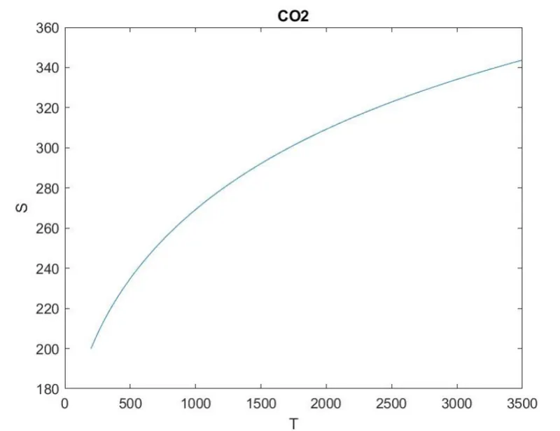
Plots of H-T, S-T and Cp-T for O2,N2 and CO2:
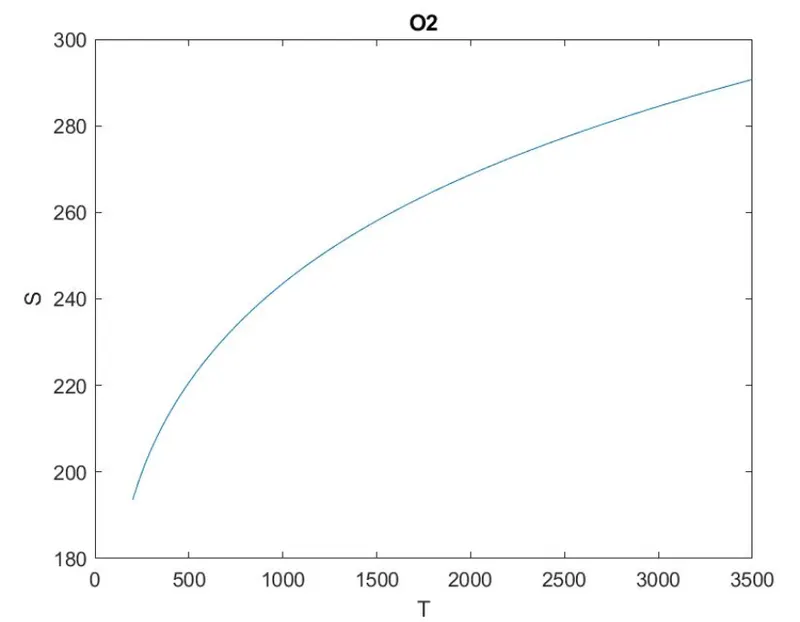
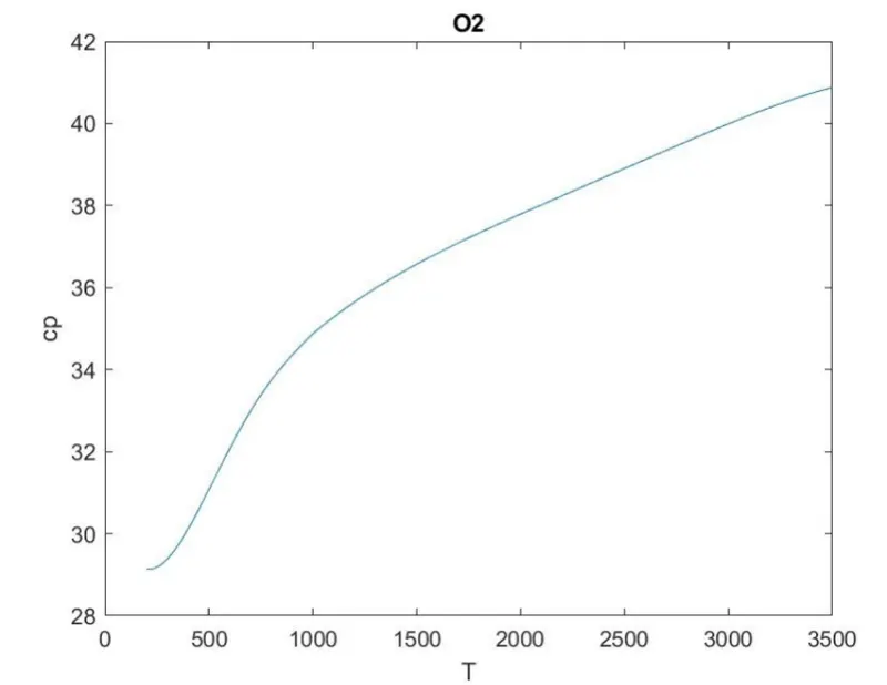
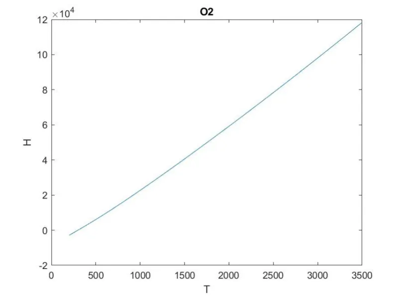
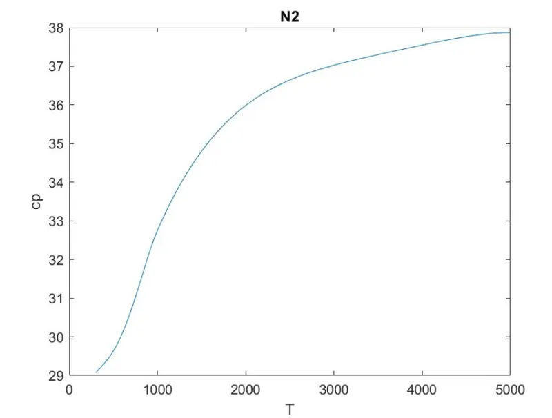
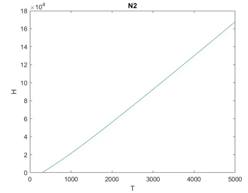
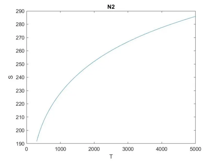
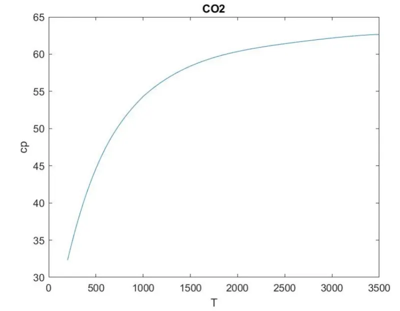
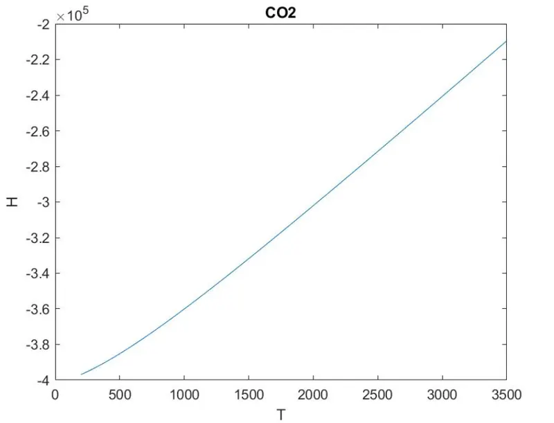
Output for molecular mass of species CH2CHO :

Errors faced :
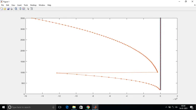
Due to incorrect definition of cp,s and H for high and low temperature co-efficients, the above graph was obtained .
On definition of the above values with proper syntax, the plots obtained were corrected.
References :