Genetic Algorithm using MatLab

Aim:-

To write code in MATLAB to optimise the stalagmite function and find the global maxima of the function.

Introduction:-

The genetic algorithm is a method for solving optimization problems that are based on natural selection, the process that drives biological evolution. The genetic algorithm repeatedly modifies a population of individual solutions. At each step, the genetic algorithm selects individuals at random from the current population to be parents and uses them to produce the children for the next generation. Over successive generations, the population “evolves” toward an optimal solution.

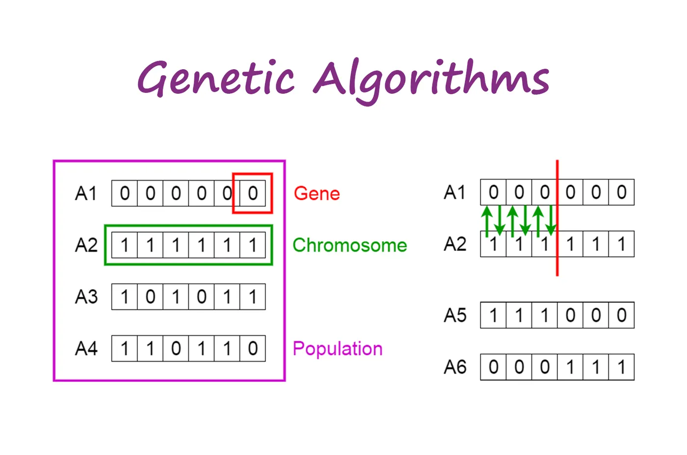
The process of natural selection starts with the selection of fittest individuals from a population. They produce offspring which inherit the characteristics of the parents and will be added to the next generation. If parents have better fitness, their offspring will be better than parents and have a better chance of surviving. This process keeps on iterating and at the end, a generation with the fittest individuals will be found.

This notion can be applied to a search problem. We consider a set of solutions for a problem and select the set of best ones out of them.

Five phases are considered in a genetic algorithm.

1. Initial population
2. Fitness function
3. Selection
4. Crossover
5. Mutation

Initial population:-

The process begins with a set of individuals which is called a Population. Each individual is a solution to the problem you want to solve.

An individual is characterized by a set of parameters (variables) known as Genes. Genes are joined into a string to form a Chromosome (solution).

In a genetic algorithm, the set of genes of an individual is represented using a string, in terms of an alphabet. Usually, binary values are used (a string of 1s and 0s). We say that we encode the genes in a chromosome.

Fitness Function:-

The fitness function determines how fit an individual is (the ability of an individual to compete with other individuals). It gives a fitness score to each individual. The probability that an individual will be selected for reproduction is based on its fitness score.

Selection:-

The idea of selection phase is to select the fittest individuals and let them pass their genes to the next generation.

Two pairs of individuals (parents) are selected based on their fitness scores. Individuals with high fitness have more chance to be selected for reproduction.

Crossover:-

is the most significant phase in a genetic algorithm. For each pair of parents to be mated, a crossover point is chosen at random from within the genes. Offspring are created by exchanging the genes of parents among themselves until the crossover point is reached. The new offspring are added to the population.

Mutation:-

In certain new offspring formed, some of their genes can be subjected to a mutation with a low random probability. This implies that some of the bits in the bit string can be flipped. Mutation occurs to maintain diversity and prevent premature convergence within a population.

Termination:-

The algorithm terminates if the population has converged (does not produce offspring which are significantly different from the previous generation). Then it is said that the genetic algorithm has provided a set of solutions to our problem.

In MatLab, There are two ways you can use the genetic algorithm with the toolbox:

• Calling the genetic algorithm function ga at the command line.
• Using the Genetic Algorithm Tool, a graphical interface to the genetic
algorithm

For this project, the ga command will be used instead of the Genetic Algorithm tool.

To use the genetic algorithm at the command line, call the genetic algorithm
function ga with the syntax:

[x fval] = ga(@fitnessfun, nvars, options) where:

• @fitnessfun is a handle to the fitness function.
• nvars is the number of independent variables for the fitness function.
• options is a structure containing options for the genetic algorithm. If you do not pass in this argument, ga uses its default options.
  The results are given by:
• • fval — Final value of the fitness function
• • x — Point at which the final value is attained

Using the function ga is convenient if you want to:

• Return results directly to the MATLAB workspace
• Run the genetic algorithm multiple times with different options, by calling ga from an M-file

Optimisation:-

An optimisation is a decision-making process, it helps to find the best results under a set of prioritized criteria or constraints. It is a procedure which is executed iteratively by comparing various solutions until an optimum or a satisfactory solution is found. These include maximizing factors such as productivity, strength, reliability, efficiency, utilization, etc.

Code:-

The code for the Fitness function is shown below in figure 2.

function [F] = stalagmite(input_vector)
x = input_vector(1);
y = input_vector(2);

f_1x = (sin((5.1*pi*x) + 0.5)).^6;
f_1y = (sin((5.1*pi*y) + 0.5)).^6;
f_2x = exp((-4*log(2))*(x-0.00667).^2/0.64);
f_2y = exp((-4*log(2))*(y-0.00667).^2/0.64);

F = -(f_1x*f_1y*f_2x*f_2y);

end

Fitness function takes the solution as input and produces the suitability of the solution as the output. This evaluates how close the solution is to the optimal solution of the desired problem.

For this project, the Genetic Algorithm optimisation process is for solving a stalagmite function, to find its minima and maxima. The stalagmite function has two inputs (x & y) as shown in figure 3 below.

The fitness function will find the value of ‘f’ by varying the sign as well as the value of the input arguments(x & y) and find the f-value that should be as minimum as possible. Now, it will compare this fitness value with the optimised value of ‘f’ for every iteration and check how good the fit is.

After defining the stalagmite function, to optimize the final program a new function was defined and its name will be “get_stalagmite” the new function contains the for loop command and mesh grid command only as shown in figure 4

function [f] = get_stalagmite(x,y)
[xx,yy]= meshgrid(x,y);

for i=1:length(xx)
for j=1:length(yy)
input(1)=xx(i,j);
input(2)=yy(i,j);
f(i,j)= stalagmite(input);
end
end

The main code for the project is shown in figure 5.

clear all
close all
clc

% Defining our search space 
x = linspace(0,0.6,150);
y = linspace(0,0.6,150);
cases = 50;

%study 1 - Statistical behaviour
f =get_stalagmite(x,y);
F=-f
tic

for i =1: cases
    [inputs,fopt(i)]= ga(@stalagmite, 2);
    xopt(i) = inputs(1);
    yopt(i) = inputs(2);
end

study1_time = toc
fopt = -fopt;

figure(1) 
subplot(2,1,1)
hold on 
surfc(x,y,F)
shading interp
plot3(xopt,yopt,fopt,'marker','o','markersize',5,'markerfacecolor','r')
title('Unbounded inputs')
subplot(2,1,2)
plot(fopt)
xlabel('Iterations')
ylabel('Function Maximum') 

%Study2 - Statistical behaviour- with upper and lower bounds

tic

for i =1:cases
    [inputs,fopt(i)]= ga(@stalagmite, 2,[],[],[],[],[0:0],[1:1]);
    xopt(i) = inputs(1);
    yopt(i) = inputs(2);
end

f = get_stalagmite(x,y)
F=-f
study2_time = toc
fopt=-fopt;

figure(2) 
subplot(2,1,1)
hold on 
surfc(x,y,F)
shading interp
plot3(xopt,yopt,fopt,'marker','o','markersize',5,'markerfacecolor','r')
title('Bounded inputs ')
subplot(2,1,2)
plot(fopt)
xlabel('Iterations')
ylabel('Function maximum')


%Study3 increasing GA iterations
options = optimoptions('ga');
options = optimoptions(options,'Populationsize',250);
f =get_stalagmite(x,y);
F=-f
tic
for i =1:cases
    [inputs,fopt(i)]= ga(@stalagmite, 2,[],[],[],[],[0:0],[1:1],[],[],options);
    xopt(i) = inputs(1);
    yopt(i) = inputs(2);
end
fopt = -fopt;

study3_time = toc



figure(3) 
subplot(2,1,1)
hold on 
surfc(x,y,F)
shading interp
plot3(xopt,yopt,fopt,'marker','o','markersize',5,'markerfacecolor','r')
title('Bounded inputs with Increased Population Size')
subplot(2,1,2)
plot(fopt)
xlabel('Iterations')
ylabel('Function maximum')

Before writing the code, it's important to start with clear all, close all and clc commands since

Clear all - removes data from the workspace, freeing up system memory

Close all- deletes the current figure or the specified figure

clc - clears all input and output from the Command Window display, giving you a "clean screen"

Two linspace commands were used to find out the values for both x and y in the search space, the number of cases was also defined as 50. f =get_stalagmite(x,y) function was used to generate stalagmite function. F=-f is used to inversing the minimum function; to get Maximum function. tic works with the toc function to measure elapsed time. The tic function records the current time and the toc the function uses the recorded value to calculate the elapsed time. The project is divided into 3 parts, the first part is for statistical behaviour. In this part, the ga command was used and the stalagmite function in figure 2 was used as the fitness function with 2 inputs. next step is plotting the graph, the subplot command was used (which creating the multiple plots in the same figure window) for the two plot windows in the same figure. the first plot is surfc(x,y, F) and using the plot3 command for x, y and the optimum value of (ga) predict's over the 50-studies. The second subplot is plotted as a function of iterations.

Results of study 1:-

Figure 6 shows the results of study 1

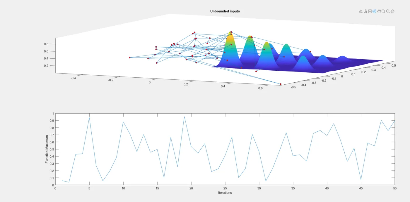
As seen in the figure the iterations look unclear hence further optimisation is required

Time taken for study 1 = 3.7948s

Results of study 2:-

For study 2, most of the steps are similar to study 1 but upper and lower bounds will be used. the syntax used is shown below where:-

[0;0] = upper and lower limit of the x.

[1;1] = upper and lower limit of the y.

Figure 7 shows the results of study 2.

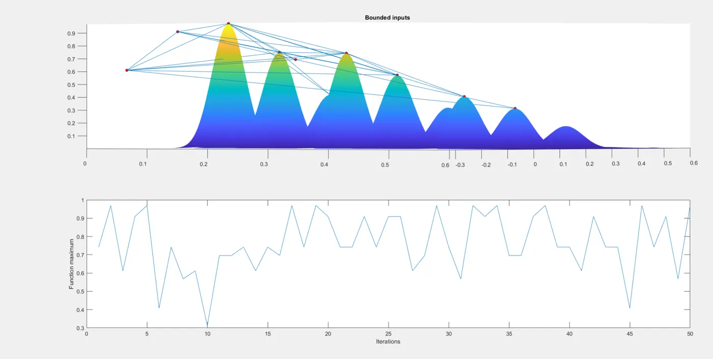
The figures look a bit more clear but still not entirely accurate, hence another optimization is required

Time taken for study 2 = 5.5130s

Results for Study 3:-

To optimize the results and getting more accuracy, the iteration number will be increased in the genetic algorithm. By default, the (ga) value is 50. The population size will be increased because if the initial population is too small then it is not going to find out global maxima (or) minima, it only finds the local maxima (or) minima. To change the ga value the following commands are used.

options=optimoptions('ga')
options=optimoptions(options,'PopulationSize',500)

Hence the ga value is now 500.

Figure 8 shows the results for study 3

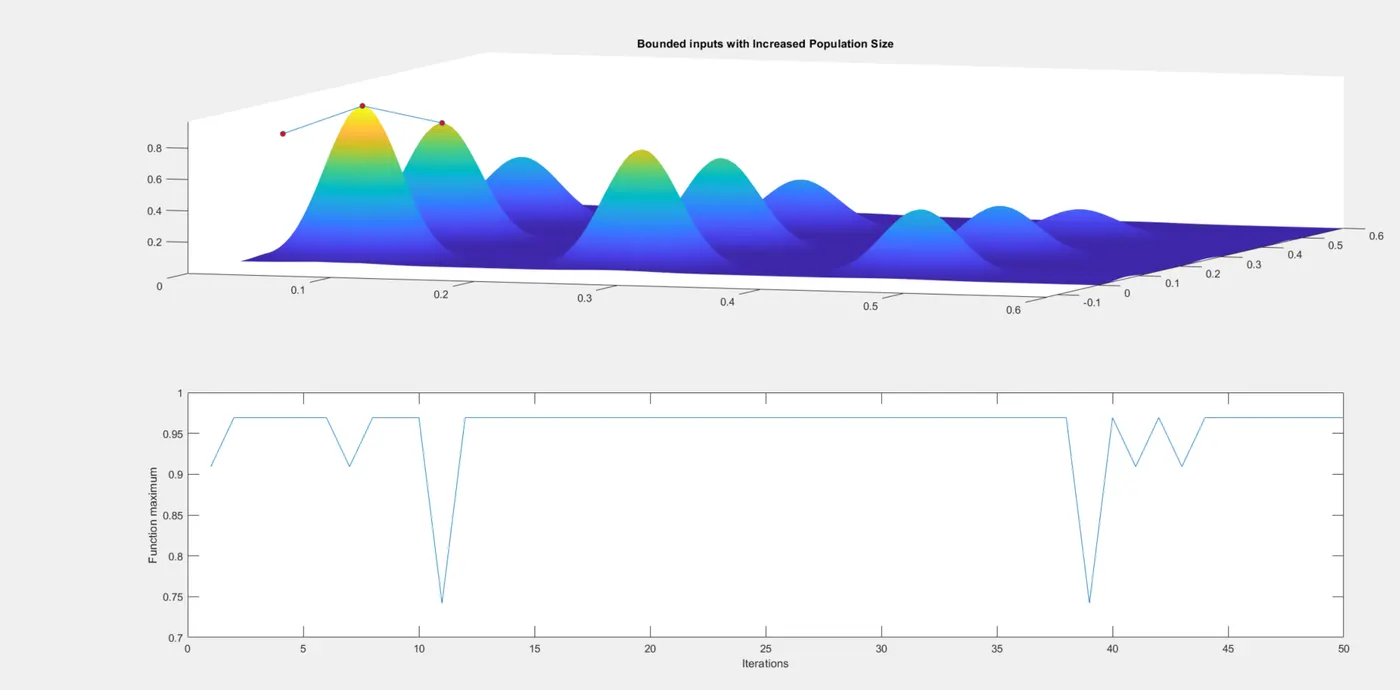
Results here are very clear and accurate.

Time taken for study 3 = 40.1553 s

Conclusion:-

The stalagmite function was optimised and used to calculate the local maxima of the function. The (ga) is only used to find the minima of the function so, therefore, to find out the maxima the function the minimum function was inversed.

The global maxima calculated is 0.9693

References:-

1. http://cda.psych.uiuc.edu/matlab_pdf/gads_tb.pdf
2. https://towardsdatascience.com/introduction-to-genetic-algorithms-including-example-code-e396e98d8bf3#:~:text=A%20genetic%20algorithm%20is%20a,offspring%20of%20the%20next%20generation.
3. https://www.mathworks.com/help/gads/examples/constrained-minimization-using-the-genetic-algorithm.html#:~:text=We%20create%20a%20MATLAB%20file,of%20variables%20in%20the%20problem.
4. https://skill-lync.freshdesk.com/support/solutions/articles/43000584189-genetic-algorithm-explained-