Week - 4 - Crash Box Simulation

AIM: To extract the model into LS-DYNA, and to create all the required keywords into the model, by creating a Rigid wall in it, with a crash velocity of 50kmph which is 13.89 mm/ms, with two different thicknesses needed to be assigned.

Objective:

1. To import the model into LS-DYNA as a k.file.
2. Once importing the model as k.file, now check for the keyword which is available.
3. Set all the required keywords and now running the model in LS-RUN.
4. Check for the Output using LS-Prepost as a binary file.

Procedure:

Import the model into LS-Dyna as k.file.

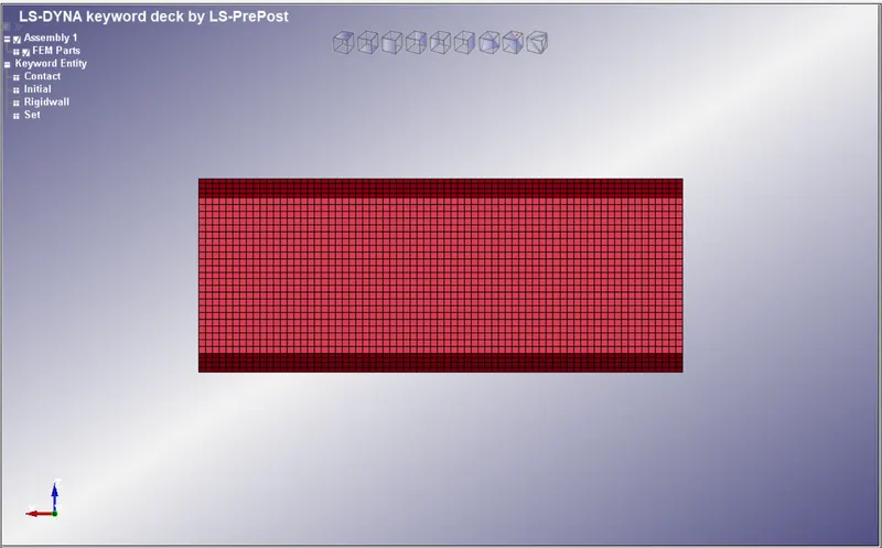
Check for available keyword

Step to create a Rigid wall in front of the Crash box, with a distance of

XT as 280, XH as 180.

YT as 80, YH as 80.

ZT as 10, ZH as 10.

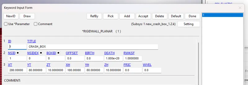
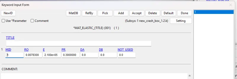
Now assign the material card by dragging all the nodes in the crash box

Here in this card, as required I have chosen Steel as a property to perform a simulation in the model.

In this unit system is considered as gm, mm, ms

E = 210*10^3; Poisson Ratio = 7.8 * 10^-3 ; Density = 0.3;

Assign Section card by choosing the master and slave nodes

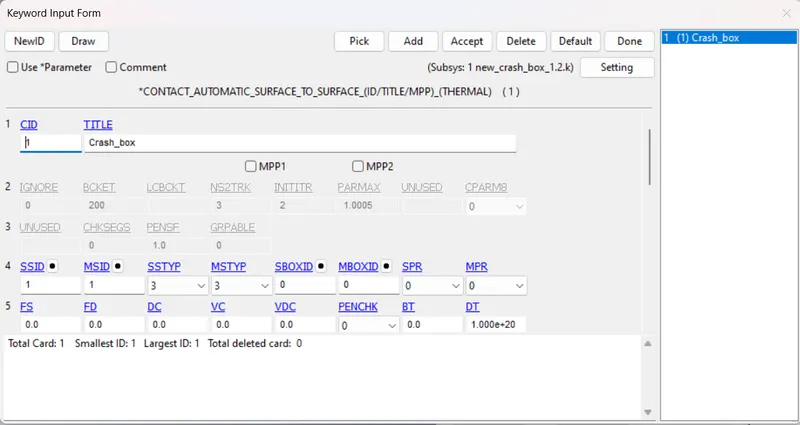
Assign Contact:

To get the result of GLSTAT, RCFORC, SLEOUT for ASCII output we need a Surface Contact, so here i have used Automatic Surface to Surface is used.

Assign Control Card:

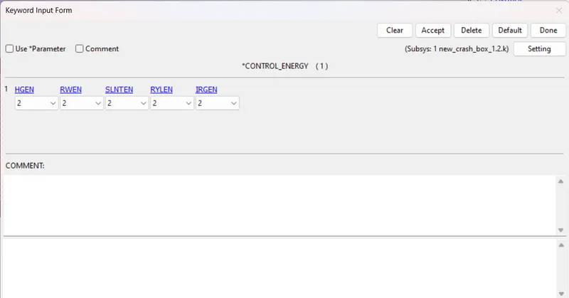
Here I used an Energy card, to assign the energy to the crash box.

Control Termination:

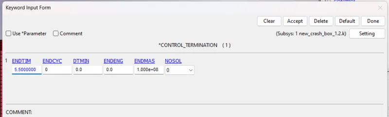
Here the termination time is a step 5.5 mm/ms, for smoother simulation.

DATABASE:

ASCII Termination Time:

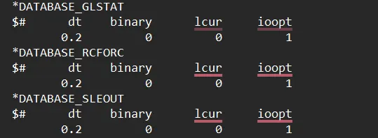
For GLSTAT, RCFORC, SLEOUT for all database termination it is set to 0.2.

D3PLOT:

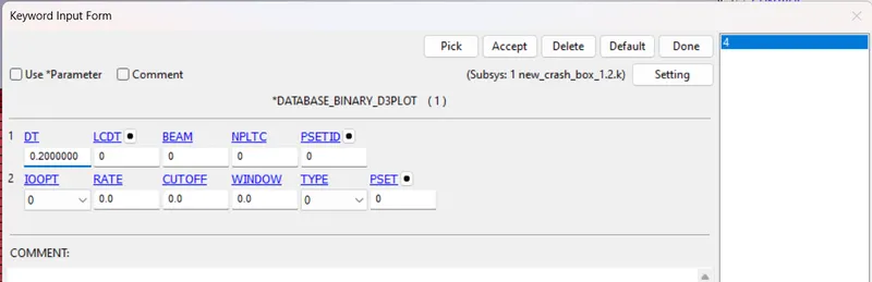
The termination time is 0.2 for the binary plot.

Velocity:

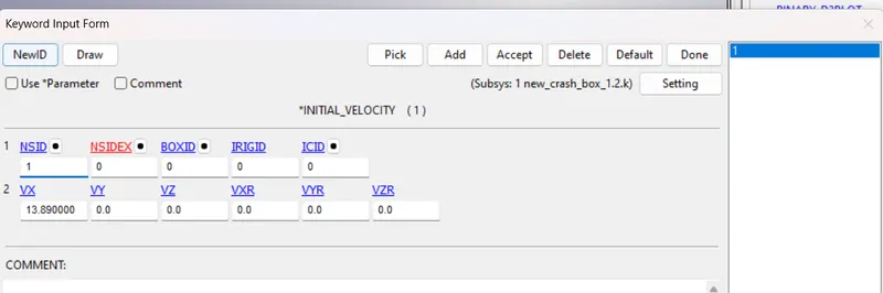
Here the initial velocity is set to 13.89 mm/ms, when we convert 50 km/h that is equal to 13.89 mm/ms. Since the flow of velocity is act on the X-axis.

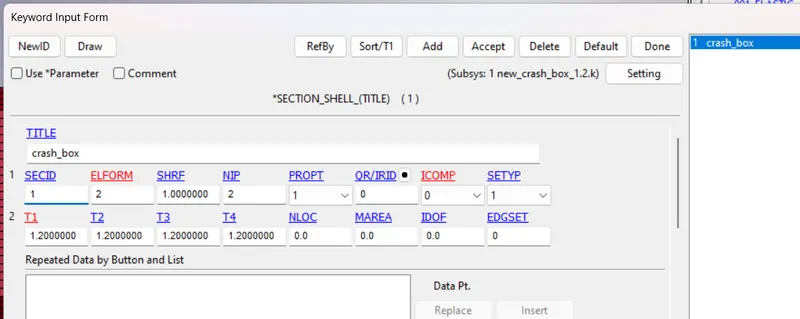
Assign SHELL:

The thickness of 1.2mm

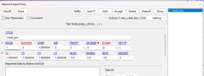
The Thickness of 1.5mm:

Now check for the model check in it.

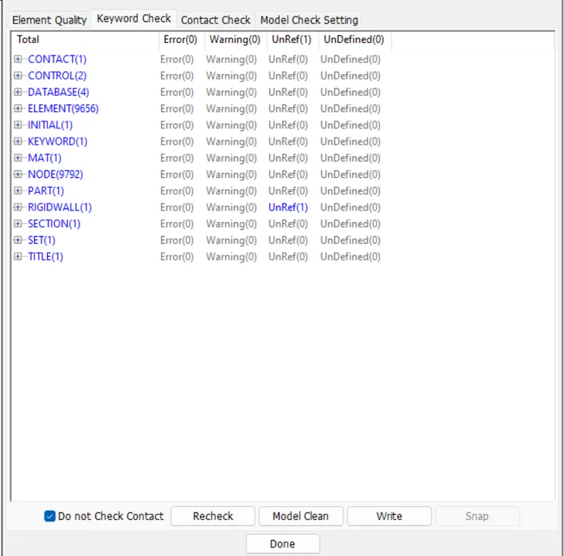
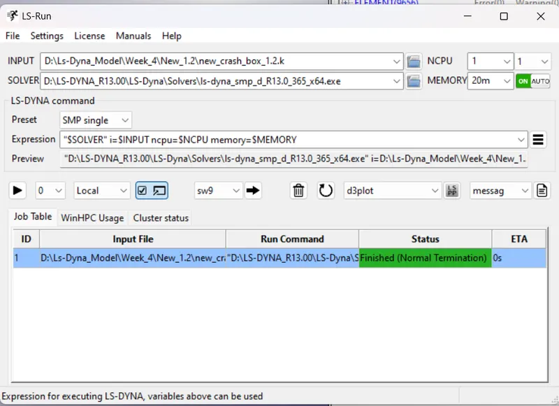
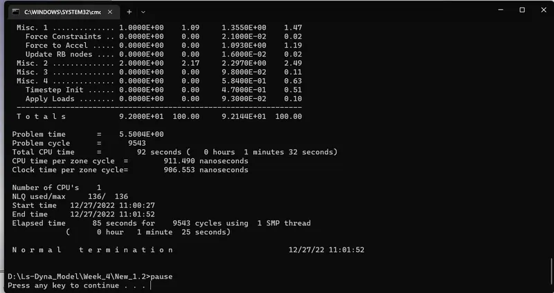
If there is no error in it, now we can run the Simulation by using LS-RUN:

OUTPUT SIMULATION:

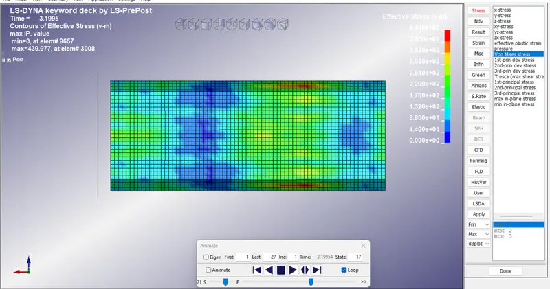
Simulation Video link:

For a Thickness of 1.2mm

https://youtu.be/fQxxq8HqFrc

For a Thickness of 1.5mm

https://youtu.be/lsHZ_pFrtUc

ASCII Output graph:

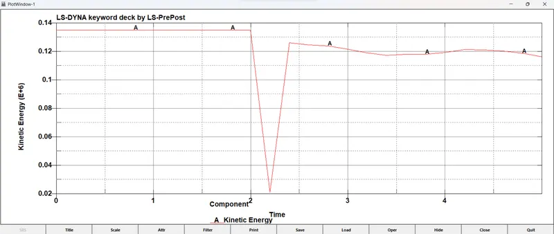
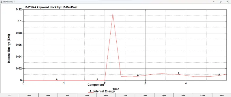
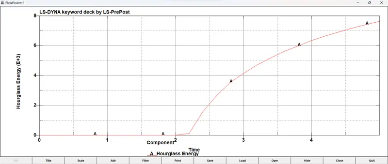
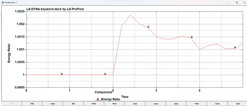
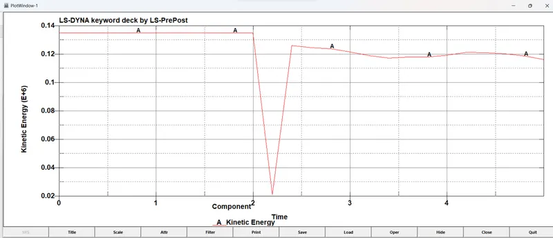
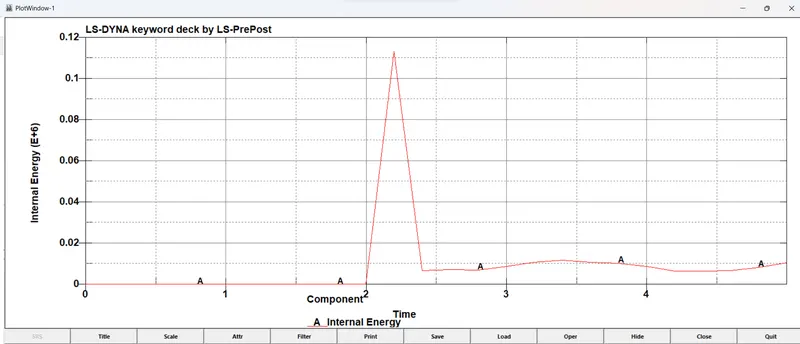
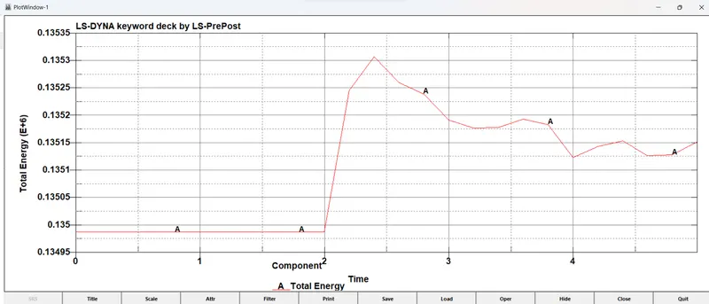
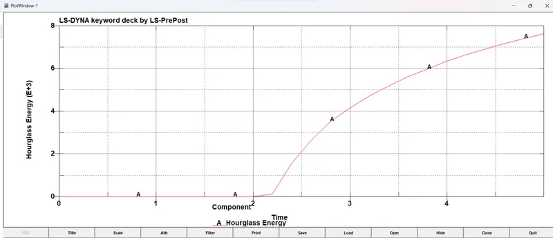
The Global Energy plots show the Kinetic energy, internal energy, Total energy, Sliding energy, and Hourglass energy values for the crash simulation.

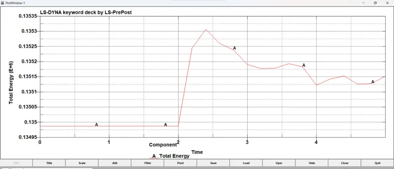
The Energies are higher for the 1.5 mm thick crash box. The total energy for the 1.2 mm thick and 1.5 mm thick crash boxes was recorded as 0.11E+6 N-mm and 0.14E+6 N-mm respectively.

At 0 ms, the whole of the total energy is Kinetic energy. But as the simulation progresses and the impact between the Crash box and the Rigid wall takes place, at approx 0.36 ms, the Kinetic energy starts getting converted into Internal energy. The Internal energy reaches its peak and the kinetic energy reaches its lowest value at about 0.44 ms when the crash box is on the verge of getting rebounded from the rigid wall. The crash box then moves with a constant rebound velocity which is reflected in the energy plot as internal energy gets converted to kinetic energy and remains constant through the rest of the simulation.

For a Thickness of 1.5mm

Total Energy:

Kinetic Energy:

Internal Energy:

Hourglass:

Energy Ratio:

RCFORC:

Resultant Force:

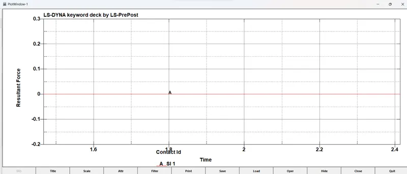
SLEOUT:

ASCII Output graph:

For a Thickness of 1.2mm

Kinetic Energy:

Internal Energy:

Total Energy:

Hourglass:

Damping Force:

RCFORC:

SLEOUT:

Conclusion:

Learned more about keywords usage, by changing the thickness of 1.2 mm and 1.5mm and studying the simulation for 1.2mm and 1.5mm with different Energy and acceleration plots.

The keywords necessary to build the crash box analysis were created from scratch.

The model was solved successfully and the results are compared for both 1.2 mm and 1.5 mm thick crash boxes.

The results of the 1.5 mm crash box showed higher energy absorbing capacity and less deformation compared to the 1.2 mm thick crash

Learned to build a solver deck for simple crash analysis in LS-Dyna and extract the outputs to interpret and compare the results.