Week - 4 - Crash Box Simulation

CRASH BOX SIMULATION

AIM :-

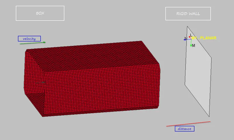
Aim of the project is setup the crash problem using shell element with elasto-plastic material with initial and imposed velocity of 50kmph and illustrate how buckling happens in body.

INTRODUCTION :-

Finite element method is good way to approximate the field variable of the governing equation. In above case(structural) we are interested in stress and strain developed in the body.

before starting the simulation we need to think about certain quation for efficitive and efficient result -

1. what method we should use for efficient solution whether implicit or explicit ?

2. how to model the material to get realistic result(elastic,plastic, hyperelastic and strain rate effect)?

3. what is the boundary condition used in model and how to simplify them(support,loads and contact)?

4. which type of element formulation(integration method) we should use(reduced , selective reduce,fully)?

5. time periodto run the simulation ?

6. what output data we need to fullfill of goal of simulation ?

7. how to verify our result in terms of accuracy ?

these are general question for most of the problem but if we answer these question then we can say our model should match with real time sinerio.

In the context of the our problem the answers are

1. the crash simulation represent the dynamic situation and for solving the dynamic problem we use explicit method for fast solution

2. in this model initially i modelled elastic matrial using youg modulus ,possoin ratio, density and after verify the simulation , i replaced the material with elastoplastic material using (effective plastive strain vs effective stress) curve.

MATERIAL PROPERTIES:

• Density: 0.0078g/mm³
• Youngs Modulus (E): 210000g/mm*ms²
• Poissons Ratio: 0.3
• Yield Strength: 571 g/mm*ms²

3. for this model i used two case

• imposed velocity
• initial velocity

and analytical rigid wall is defined using rigidwall keyword and self contact is defined

4. element formulation is really important in finite element analysis. generally we have element formulation broadly classified on the basis of the integration point

• full integration method
• reduced integration method
• selective reduced integration method

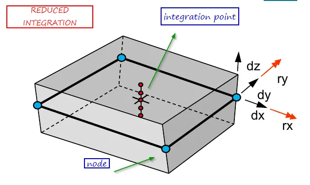
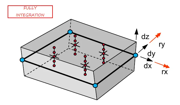
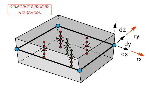
fully integration is accurate but there is issue of shear locking and volume locking. solving the shear and volume locking we use reduced integration but using reduced integration leads to introduction of hourglass energy. so hourglass control must be used

hourglass can be control by two ways

• introducing excess stiffness to the nodes
• introducing the viscous effect

in this case reduced element formulation for shell element is usedand stiffness method is best for houglassing control.

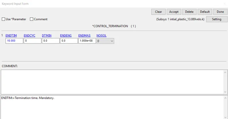
5. time period for simulation is calculated by 2 times of

time = distance/velocity

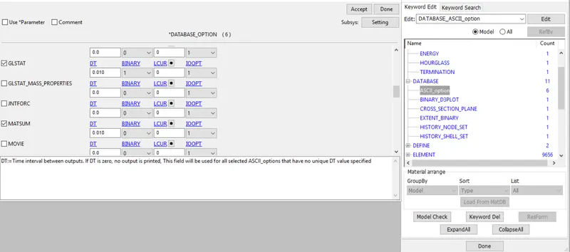
6. in this case i enable the global energy data(glstat), material data(matsum) ,reaction force data(rcforce)

7. model can verify using energy plot total , internal, kinetic , hourglass ,sliding

UNIT SYSTEM USED: G MM MS

PROCEDURE:

1. Importing:

• FILE > OPEN > LS DYNA KEYWORD FILE > NEW_CRASH_BOX.

after importing the model it is required to check keyword and then check for duplicate element.

2. define section for shell element :

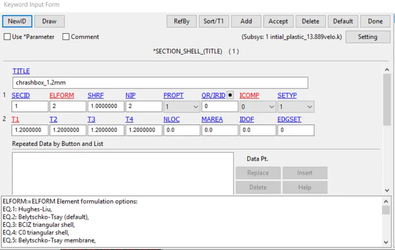
3. define material using "mat_elastic" card :

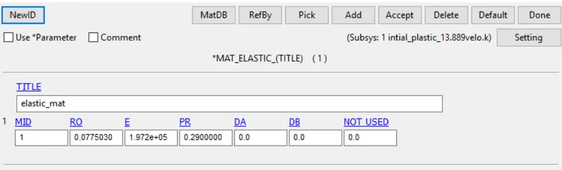
4. define section card to part :

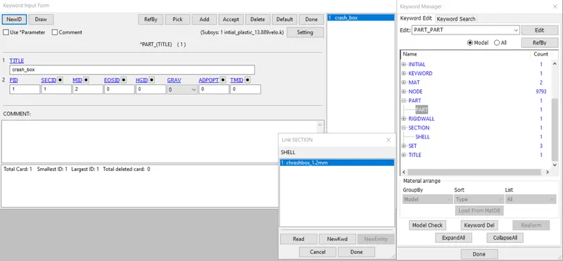
5. define material card to part :

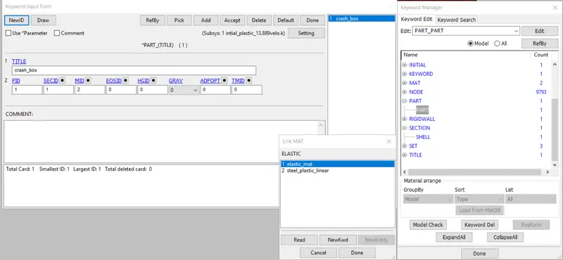
6. define rigid wall

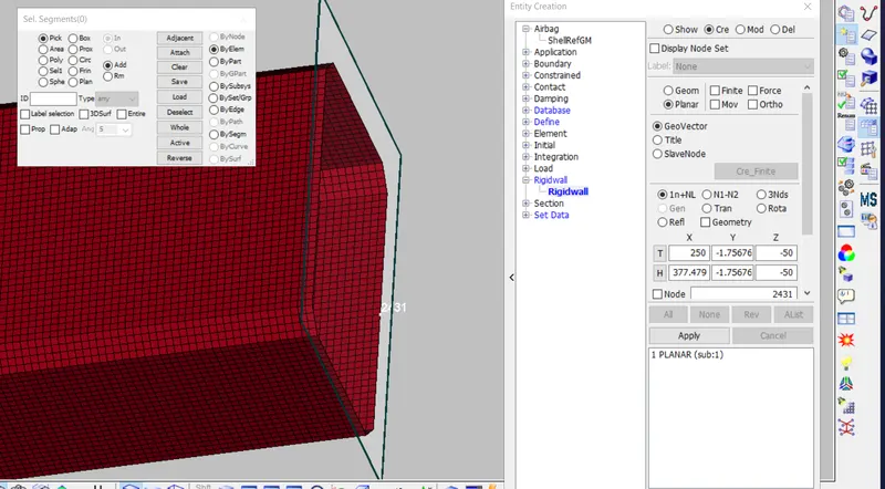
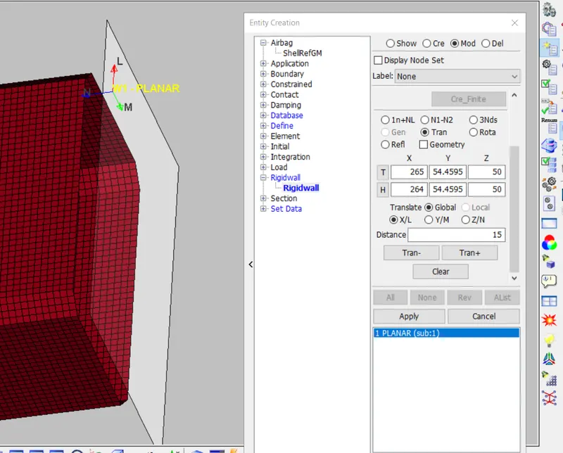
after creation of the rigid wall it is required to translate the rigid wall

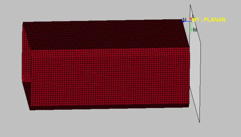
normal vector of the rigid wall plane should be in direction of the body as shown below otherwise it will not treat contact between wall and box

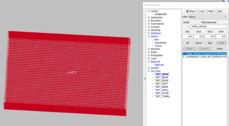
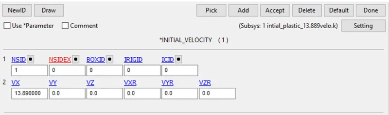
7. define initial velocity

50kmph =13.889 mm-ms

define the node set for which velocity should applied

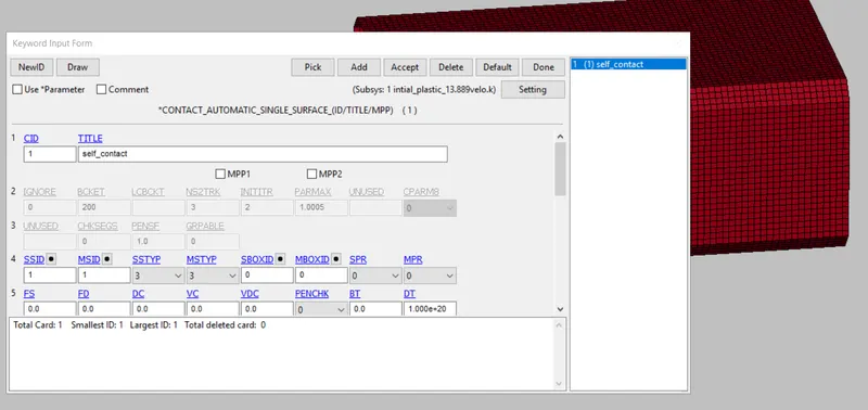
8. defining the contact

self contact is defined for box surface itself to predict proper buckling effect if happens

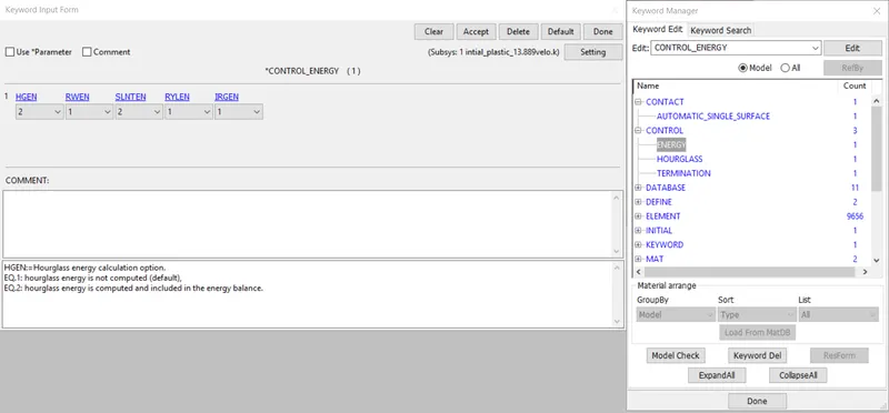
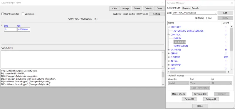
9. energy modes allow

we used the reduced integration point formulation which introduce the hourglass in the simulation. reduction the effect of hourglass is necessary. for this enable the hourglass mode using the ENERGY card from control keyword and enable the HOURGLASS card from control keyword, set IHQ = 5, QH = 0.03

10. time period for simulation

11. enabling the Output data

enable the energy output using glstat, matsum

reaction force using rcforce

animation using binary D3PLOT

now our setup is ready for running the simulation then save the file

PLASTIC MATERIAL

now after verify the model with elastic material then model with plastic behaviour using the MAT_24 card

first define the curve between effective plastic strain and effective stress

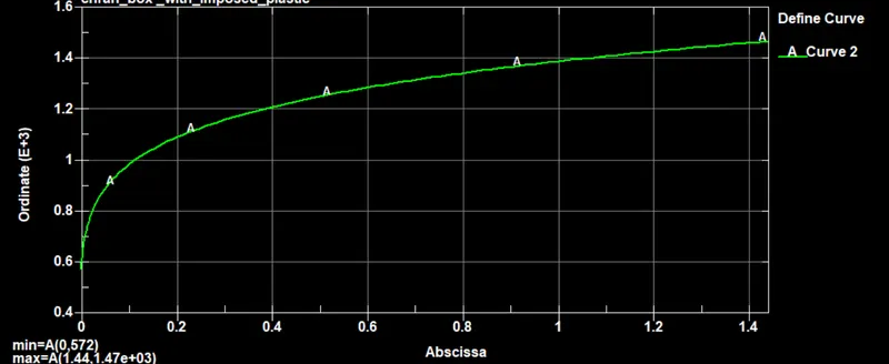
link this curve in the MAT_24 byLCSS

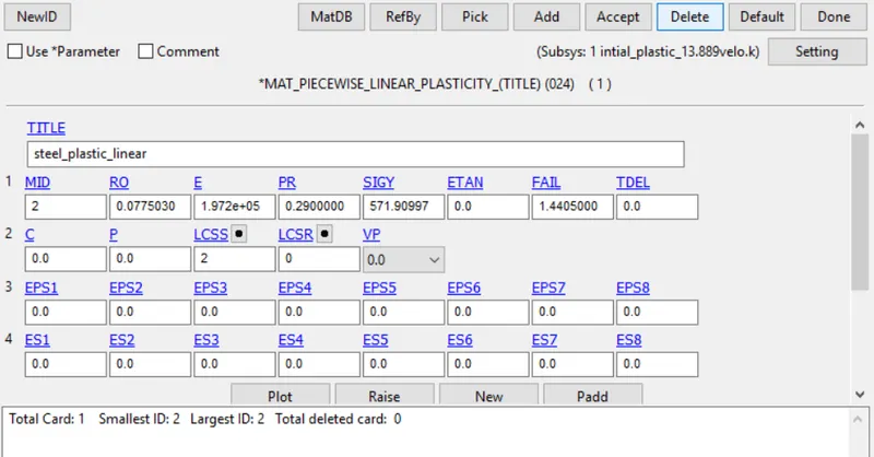
after the modelling the material we just need to link the material(MAT_24) with the part instead of elastic

IMPOSED VELOSITY

all the steps are similliar as above but difference is defininig the velocity boundary condition. Instead of defining the initial velocity we used imposed velocity

step for defininf the imposed velocity

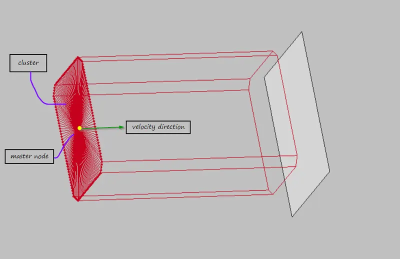
1. define the node set(rigid) at the end face of the body and make the master node at the center of the cluster

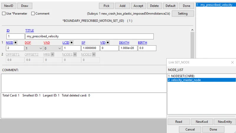
2. define PRESCRIBED_MOTION_SET card from boundary keyword

apply the velocity profile using using curve by LCID

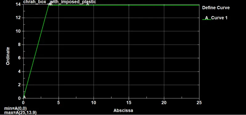
now our imposed velocity with 13.889 mm-ms is defined

now using the combination of velocity condition(initial,imposed) and material type(elastic,elasto-plastic)

we can create different different simulation setup like

• elastic with imposed velocity
• plastic with initial velocity
• plastic with imposed velocity

and compare the result from different simulation

simmiliar way model can be setup for different thickness 1.2mm and 1.5mm

POST PROCESSING :

elastic with initial

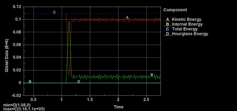
elastic with imposed

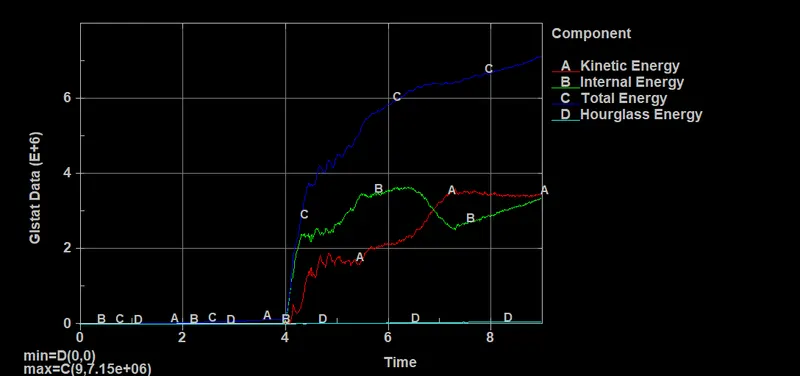
plastic with initial

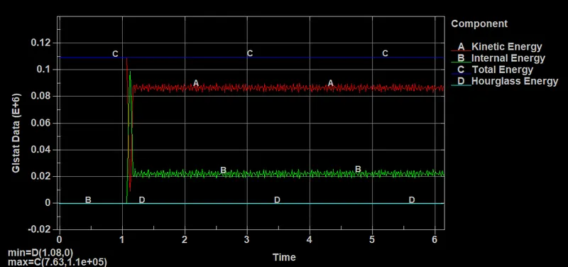
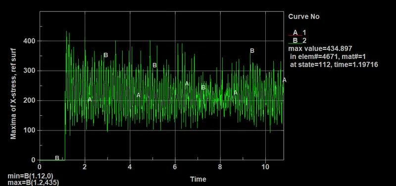
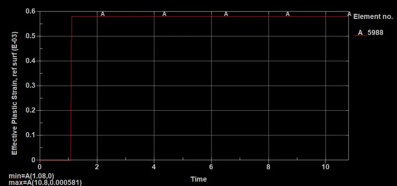
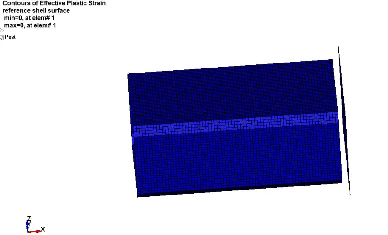
plastic with imposed

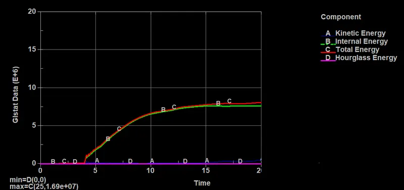
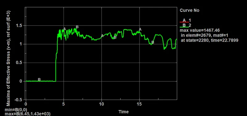
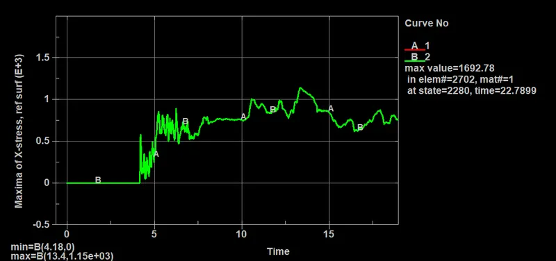
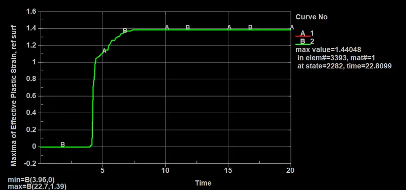
the comparision stress and strain at different section with plastic material and intial velocity condition

	Max-Stress(MPa)			Max-Strain
Model Thickness	X-Direction	Y-Direction	Z-Direction	X-Direction	Y-Direction	Z-Direction
1.2 mm	276.08 on Ele 5706	264.5 on Ele 5984	263.01 on Ele 9523	0.00118 on Ele 5707	0.00127 on Ele 5980	0.00127 on Ele 1498
1.5 mm	247.45 on Ele 3012	236.33 on Ele 6973	227.69 on Ele 105	0.00126 on Ele 3000	0.00126 on Ele 5987	0.00123 on Ele 1263

CONCLUSION

1. The model was solved successfully and the results are compared for both 1.2 mm and 1.5 mm thick crash box.
2. The results of 1.5 mm crash box showed higher energy absorbing capacity and less deformation compared to 1.2 mm thick crash
3. Learned to build a solver deck for simple crash analysis in LS-Dyna and extract the outputs to interpret and compare the results.