Week - 4 - Crash Box Simulation

- Input .k file and output files (d3plot, glstat, sleout, rcforc)

- Animation of the final simulation

- Cross-sectional force generated in the middle of the crash box (along its length)

- Acceleration plot of a node in the middle of the crash box (along its length)

- Maximum directional stress and strain along the length of the crash box (X strain, Y strain etc)

- Plot of all energies (total, internal, kinetic, hourglass, sliding)

- Compare the accelerations and stress/strain plots of 1.2/1.5mm crash boxes.

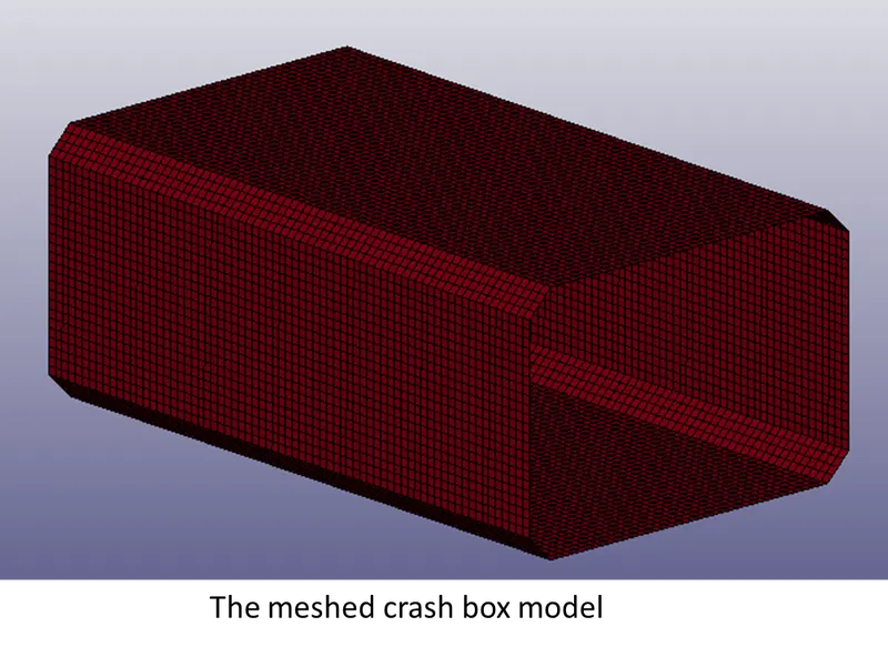
Fig 1.1: The meshed model provided as a keyword file.

The crash box is supposed to crash on a wall and there is no wall in the model, we need to model one for getting the right set up. This was done using the rigid wall option available in the entity creation window of the LS- Pre-Post. It was translated to place it at a 10 mm distance from the crash box.

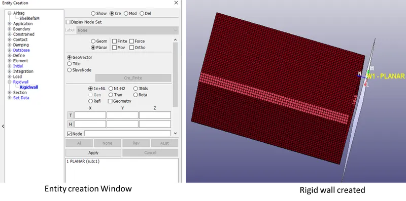
Fig 1.2: Rigid wall creation process

After that, we need to add all the essential data cards to the model. For the starting point, a general elastic material with properties of steel was modelled using the 001 elastic material card as shown in the below-attached figure.

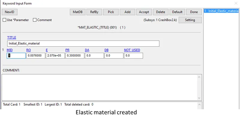
Fig 1.3: The 001 Elastic material card used to model a simple elastic material.

After that, we need to define section properties for the crash box model. Shell card was used with settings as shown in the attached figure.

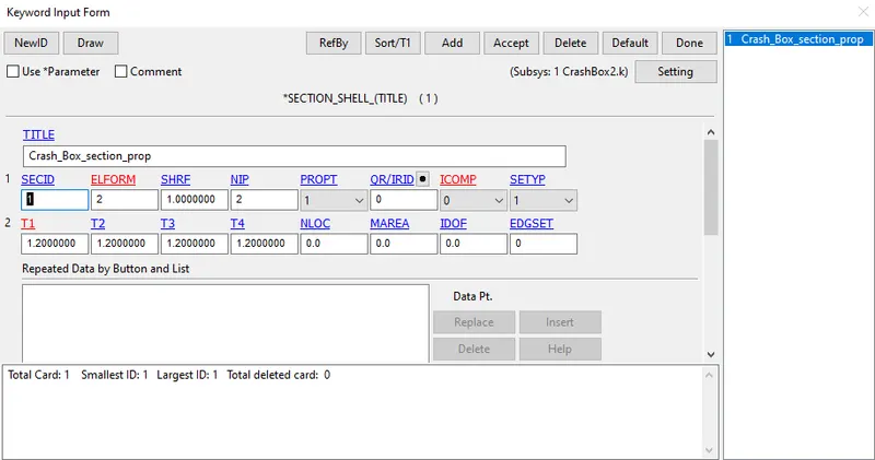
Fig 1.4: The shell section card is used to define section properties for the model.

As we used Element formulation =02, an hourglass card can be provided to control hourglassing during deformation. For this purpose, the Flanagan-Belytschko viscous form was used by setting IHQ= 2.

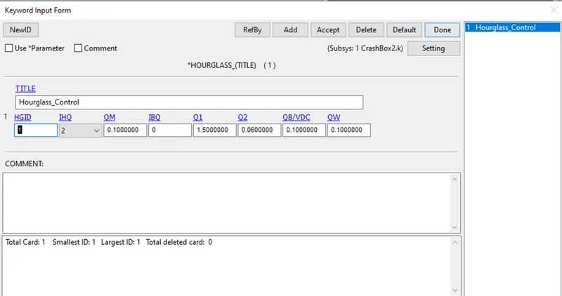
Fig 1.5: The hourglass card used for the model.

Next, we need to provide the initial velocity to the crash box model. This was done using the entity creation tool as shown in the attached figure.

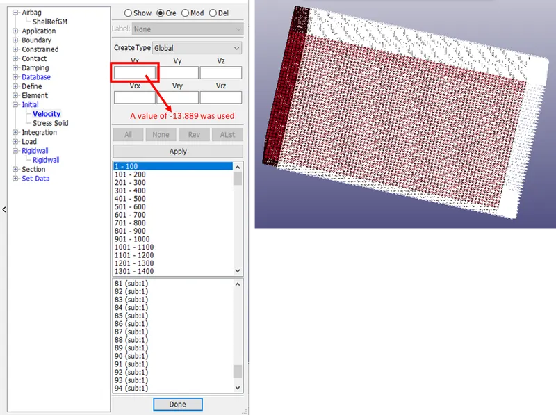
Fig 1.6: The entity creation window used for creating the initial velocity.

After this, we need to provide a self contact card for the model to be able to deform and avoid penetrating into itself during the impact. This was done using the contact_automatic_single surface card as shown in the attached figure.

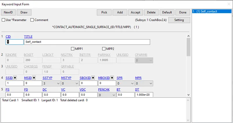
Fig 1.7: The single surface contact card used in the model.

All the contact definitions in LS-Dyna needs a slave and master to be defined. Master and slave selection is based on the relative stiffness of the components, a stiffer material is chosen as master and the softer one is deemed as a slave for the contact. In the case of the single surface card, only the slave part needs to be selected. The selection was made by setting SSTYP to part mode and then selecting the part ID of the crash box in the SSID box.

Then the control_termination card was used to define simulation runtime. The unit used was [g-mm-ms] so a value of 2 ms was used for simulation time. The calculated time of impact taking 10 mm gap and 13.889 mm/ms velocity is 0.72 ms so we kept the simulation time larger than this value so as to capture the entire phenomena.

Mainly there are two types of output files that can be requested; binary and ASCII. Binary files include all the stress-strain related data and are present in the name of D3plot in the keyword list. A DT value which means recording interval for the requested output needs to be specified. In our case, it was set to 0.01 ms. In ASCII options the GLSTAT, NODEOUT, ELOUT, MATSUM and SECFORC were requested at every 0.01 ms. Apart from this, for the secforc to be generated we need to define sections in the model which was done using the create entity window.

History_node_set card was used to get all the details about nodes in the middle of the model.

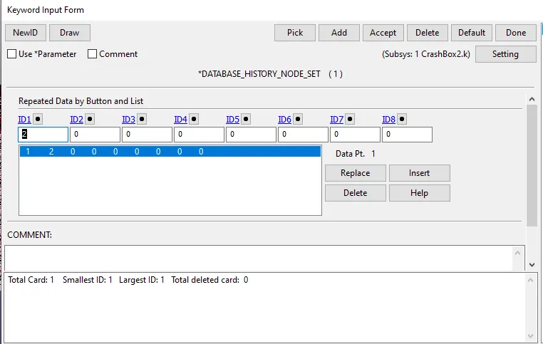
Fig 2.1: The History_Node_Set card used in the model.

Animation 3.1.1: The crashbox simulation with simple elastic material.

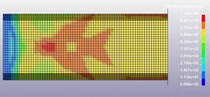
Fig 3.1.1: The stress plot right after the impact.

As clear from the above the max value of Von Mises Stress is 713.405 MPa. Also, in the animation, the stress pattern clearly shows the high-stress value at the interface and its flow to other areas as time progresses.

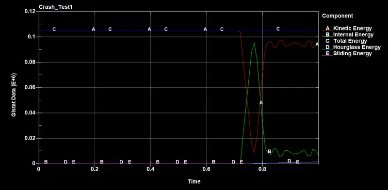
Fig 3.1.2: Plot of energies for the model.

As clear from the above plot, the total energy remains conserved and hourglass and sliding energy are negligible which tells us that the results are ok.

This simulation was just an initial check with the linear material card. After this, a non-linear material card Mat_024 which is Piecewise linear plasticity material model was used to run two more simulations as explained in the following sections.

3.2 Crash Test with 1.2 mm thickness and Mat 024 Piecewise Linear plasticity model.

This time the material used was changed to a piecewise linear plasticity model with values from a typical steel property. The values used are shown in the attached figure and tangent modulus was set at 1% of Young's Modulus. Also, the simulation run time was increased to 2 ms for better visualisation of the phenomena.

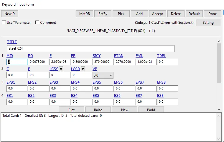
Fig 3.2.1: The 024_material card used for modelling a non-linear elastic material.

Rest all the settings were kept the same and simulation was run. The results are discussed in the below section.

Animation 3.2.1: The stress contour animation of the crash box with 1.2 mm thickness.

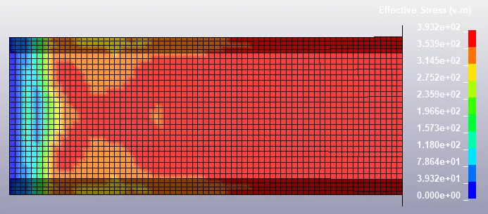
Fig 3.2.1: The stress plot right after the impact

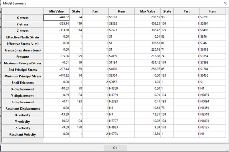
Fig 3.2.2: The summary of the model output

From the above summary table, it is clear that the maximum directional stress is 440.32 MPa. The strain values are negligible because of the fact that deformation is very low as the gap between the rigid wall and the crash box was not very much.

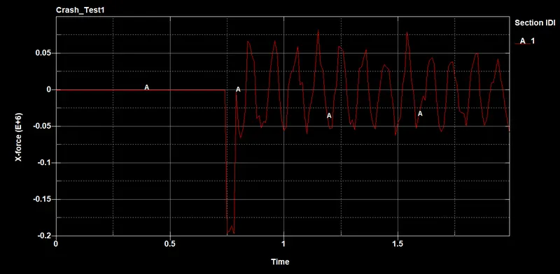
Fig 3.2.3: The plot of section force generated at the middle section of the crash box.

A peak in the negative direction represents the compression of the cashbox in the X direction during impact.

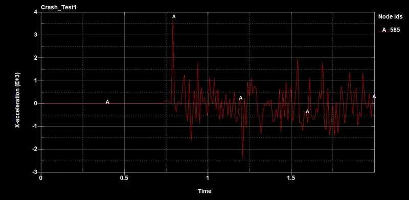
Fig 3.2.4: the acceleration plot of a node in the X direction

A peak around 0.7 ms represents impact and subsequent vibrations are shown by fluctuation in the values.

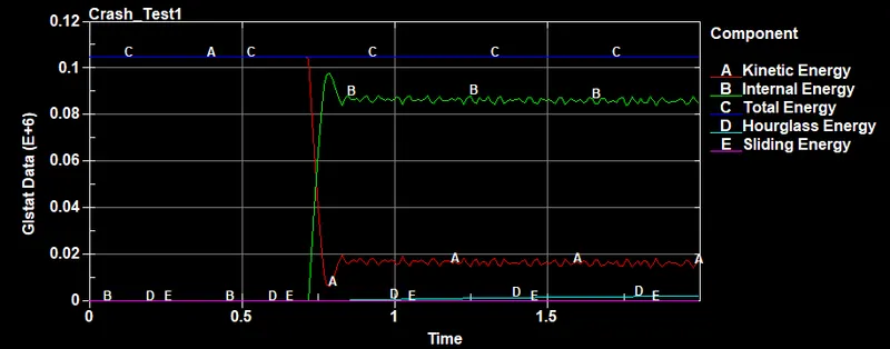
Fig 3.2.5: The plot of various energies for the model

As clear from the above plot the hourglass and sliding energies are very low in comparison to the other energies, we can safely say that the simulation was ok and it served the purpose.

This time the thickness of the crash box was changed to 1.5 mm and simulation was run by keeping everything else the same.

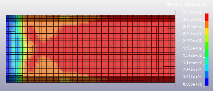
Fig 3.3.1: The stress plot for the 1.5 mm thickness model of the crash box.

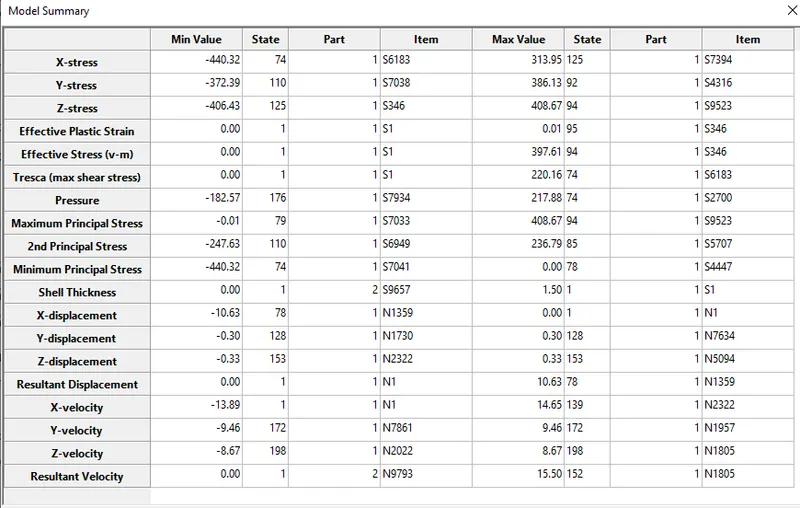
Fig 3.3.2: The model summary depicting all the values

Fig 3.3.3: the section force plot for the cross section created in the middle of the model.

A very minor difference can be observed in the values as compared to the plot obtained for the 1.2 mm thick plate.

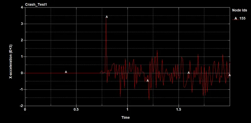
Fig 3.3.4: the acceleration plot for a node in the middle of the model plotted in x direction values.

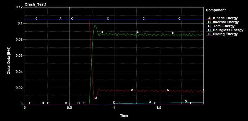
Fig 3.3.5: Plot of various energies for the 1.5 mm thickness model

As clear from the above plot the hourglass and sliding energies are very low in comparison to the other energies, we can safely say that the simulation was ok and it served the purpose.