Week 4 - CHT Analysis on Exhaust port

Aim:-To study the Conjugate heat transfer analysis of exhaust port using Ansys fluent.

Objectives

The objective of the simulation are

How would you verify if the HTC predictions from the simulations are right? On what factors does the accuracy of the prediction depend on?

Theory:

CHT Analysis:

• Conjugate heat transfer analysis describes heat transfer as a result of interaction between a body and a fluid that is flowing over a inside it.
• This type of heat transfer includes both convection (between fluids)and conductive (between solids) heat transfer, as well as both forced and natural convection.
• At the matching interface, the details are provided for temperature distribution and heat flux along the interface eliminating the need of calculating the heat transfer coefficient, moreover the heat transfer coefficient can be calculated later.
• Conjugate heat transfer is important for designing effective coolers, heaters and heat exchangers. for example, in a heat exchanger, solid separate fluids so that they can exchange energy without mixing.
• One of the simplest ways to realize conjugation is through numerical methods. The boundary condition for the fluid and solid interface is set and solved through iteration methods. There are no right guesses for the values of the initial boundary condition for the convergence except through the hit and trail method.

Application of CHT Analysis:-

• Conjugative heat transfer(CHT) analysis is used in many real-world applications to simulate heat transfer between solids and fluids. the CHT methods have become a more powerful tool for modeling and investigating natural phenomena and engineering systems in different areas ranging from aerospace and nuclear reactors to thermal goods treatment and food processing from the complex procedures in medicines to ocean thermal of metrology.
• CHT analysis commonly used to simulate the cooling of electronic equipment, such as heat sinks and heat exchangers. CHT analysis helps determine the rate of heat transfer between the coolant fluid and solid walls of heat exchangers used in refrigeration, air conditioning, and electronics. CHT analysis considers both conduction in solids and convection in fluids. CHT analysis is used to simulate the temperature distribution in brake components influenced by airflow convection.

Y+ Value:-

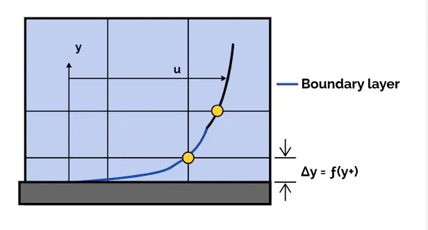
• The y+ value is a non-dimensional distance from a wall to the first mesh node in computational fluid dynamics(CFD). It's used to describe the coarseness or fineness of a volumetric mesh for a flow pattern. The y+ value is important for modeling turbulence because it helps determine the proper size of mesh cells near no-slip walls.
• To calculate the boundary values accurately the mesh needs to be finer at the boundaries. The y+ value is an important parameter for determining the accuracy of the boundary layer thickness. The y+ value can help estimate how many cells are needed to resolve the viscous sublayer. A low y+ value indicates laminar flow, while a large y+ value indicates turbulent flow.

Simulation(Baseline Mesh):-

Geometry:-

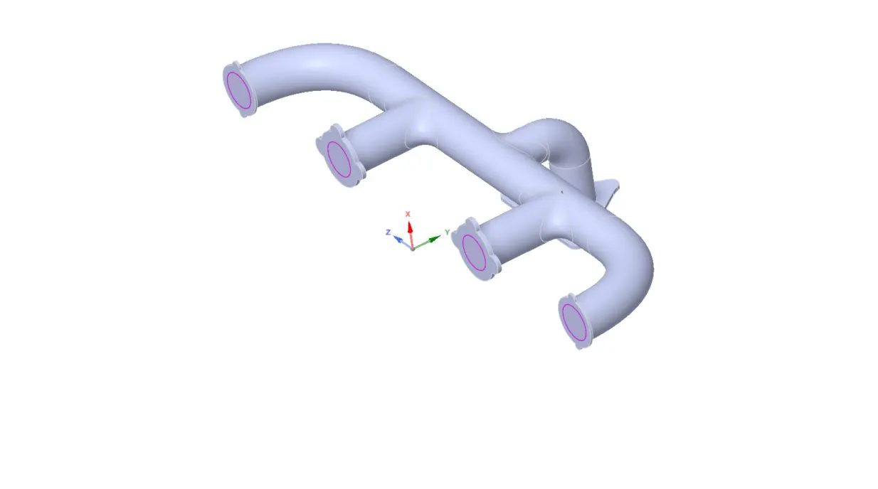
The exhaust port .step file is imported to SpaceClaim. The exhaust port is a three dimensional model containing four inlets and one outlet. After that the fluid volume is extracted by using volume tool.

CHT analysis requires both the solid and the liquid volume under consideration, so both the solid volume and liquid volume are copied into one component.

share topology is created, which allows information to be shared between the fluid and solid volume.

To make sure there is only one interface between solid and fluid volume, the share prep tool is used.

Meshing:-

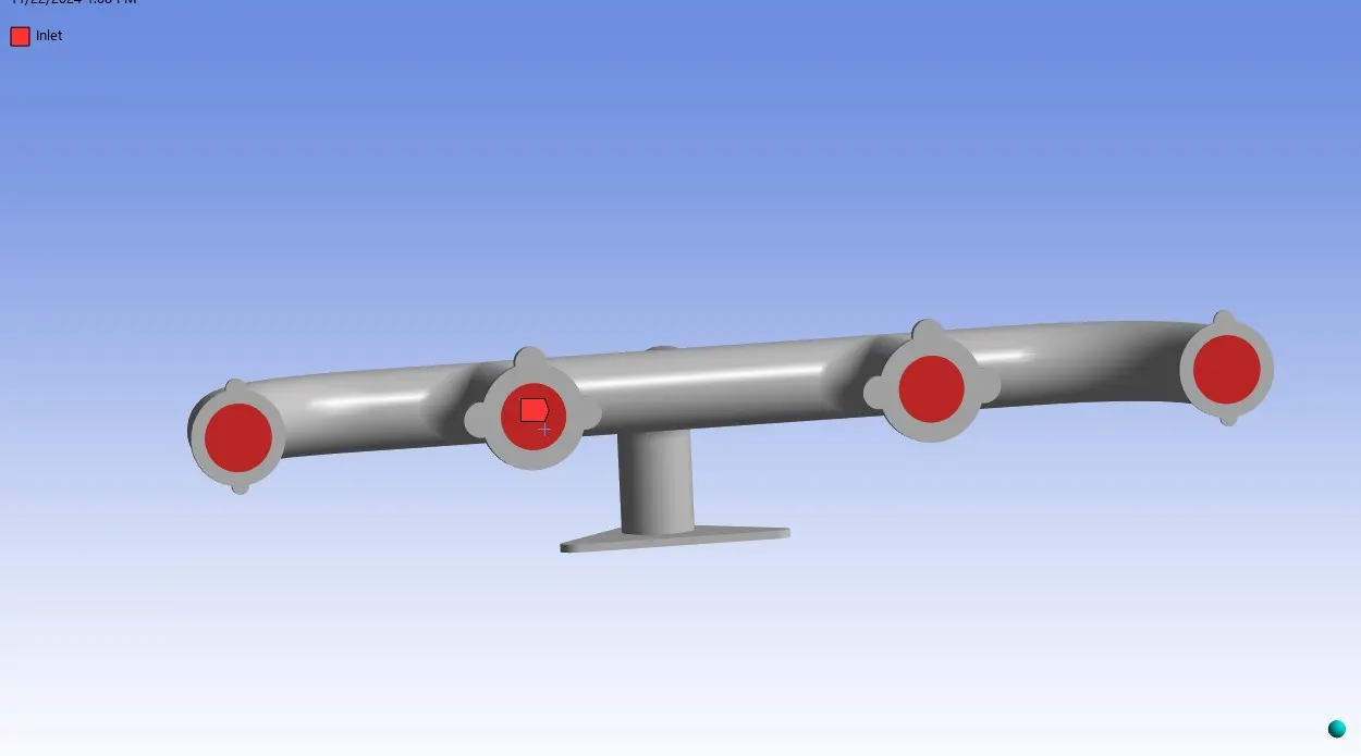
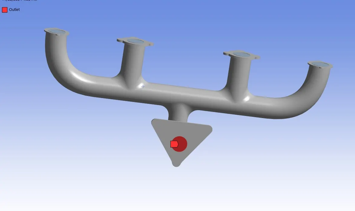
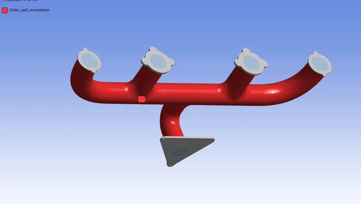
Then we close spaceclaim. The named selections are created as follows,

inlet

Outlet

Outer_wall_convection

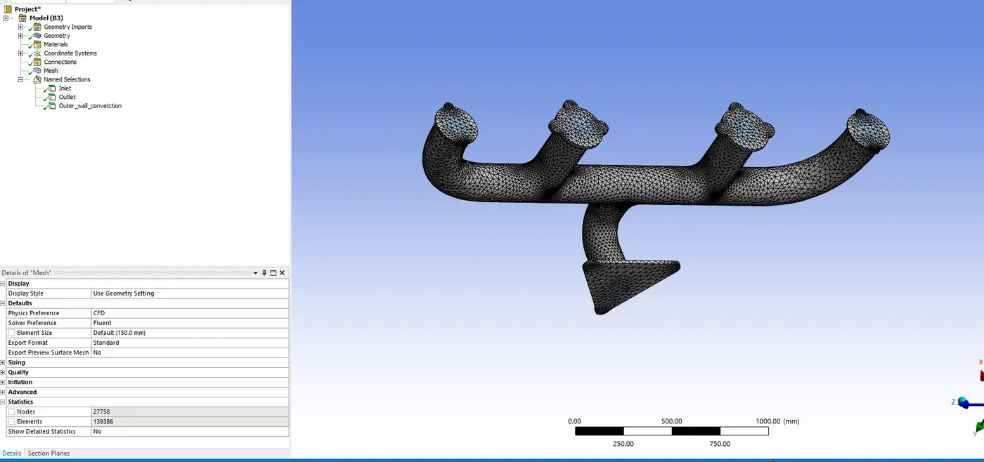
For the baseline simulation, we use the default mesh size. then we did generate mesh and check if the mesh from solid volumes are in sync. then we checked also mesh quality.

Setup-fluent:-

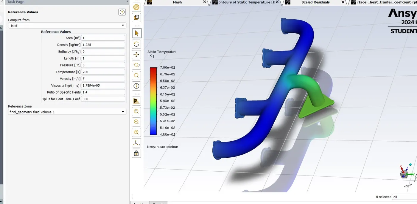
The meshed geometry is loaded in ANSYS fluent. for this simulation, the pressure-based solver is used. the steady state is considered, the reference values are updated. we use it for baseline simulation. the energy equations are included, The default air is used for fluid material and aluminum is used for the solid material, the inlet (velocity)=5m/s and temperature=700k,The outlet is a pressure boundary. for the outer surface of the pipe, the convection boundary condition is used. The heat transfer coefficient for the wall, h=20w/m2k is assigned after verifying with the analytical value.

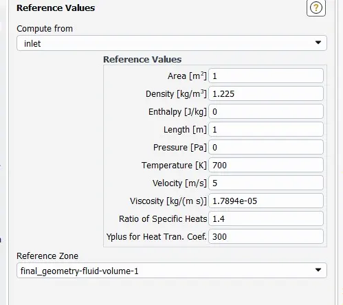
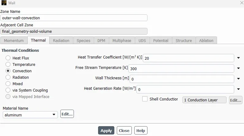
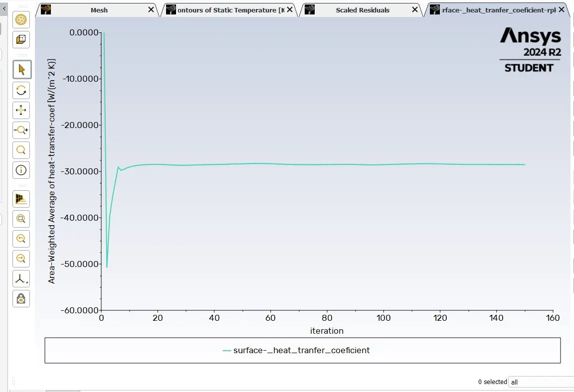
Area weighted average of the surface heat transfer coefficient for the internal surface of the pipe is defined, then

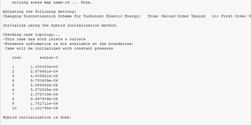
Then hybrid initialization is performed to enable create a contours tool.

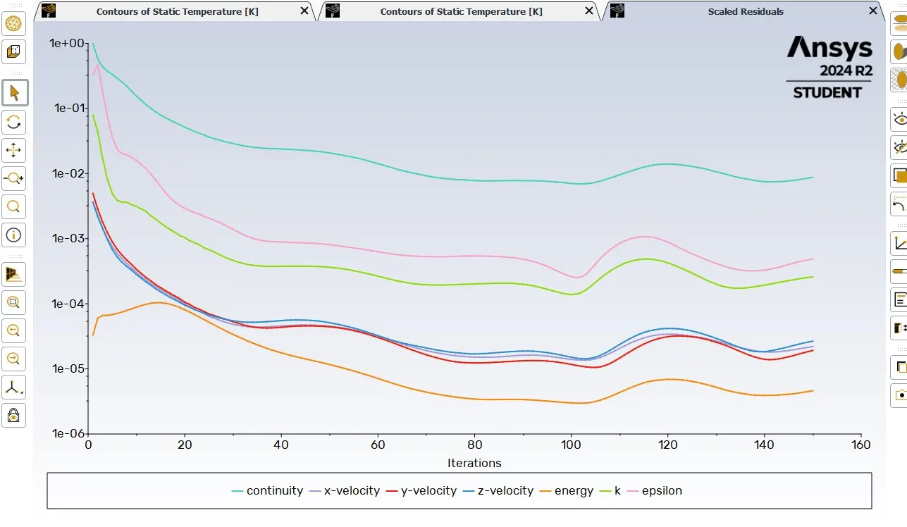
The temperature contour is created and the animation contour is created for the same, Then the simulation is performed foe 150 iterations.

Results:-.

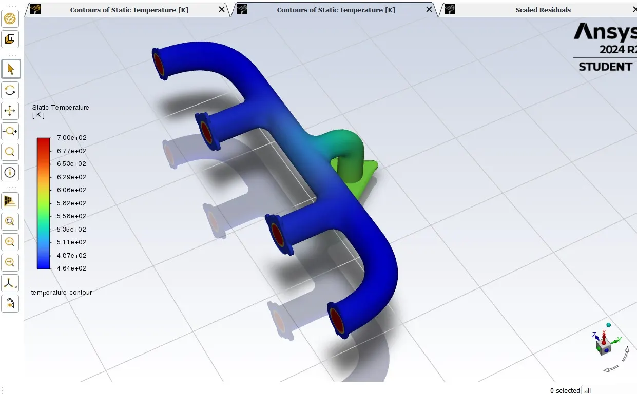
The temperature contour and the surface heat transfer coefficient plot are generated here.

residual plot:-

Temperature contour:-

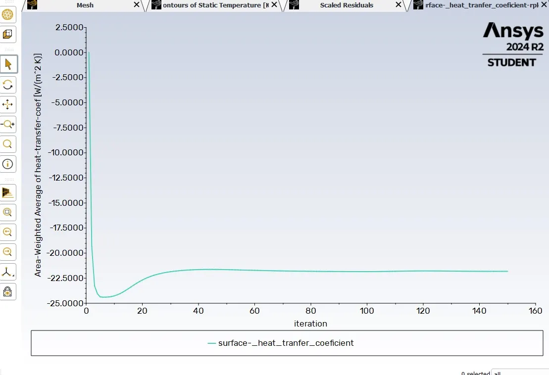
Surface heat transfer coefficient on the internal solid surface plot:-

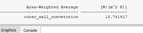
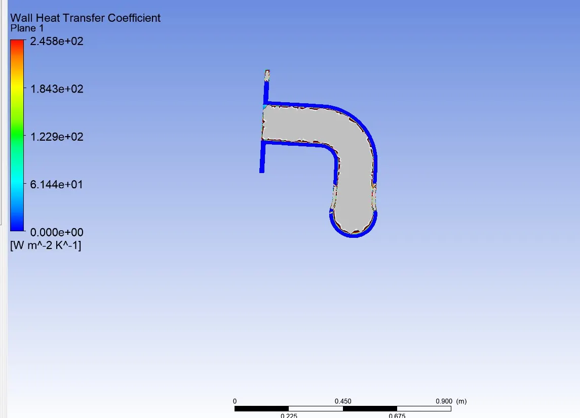
The outer surface heat transfer coefficient is also calculated

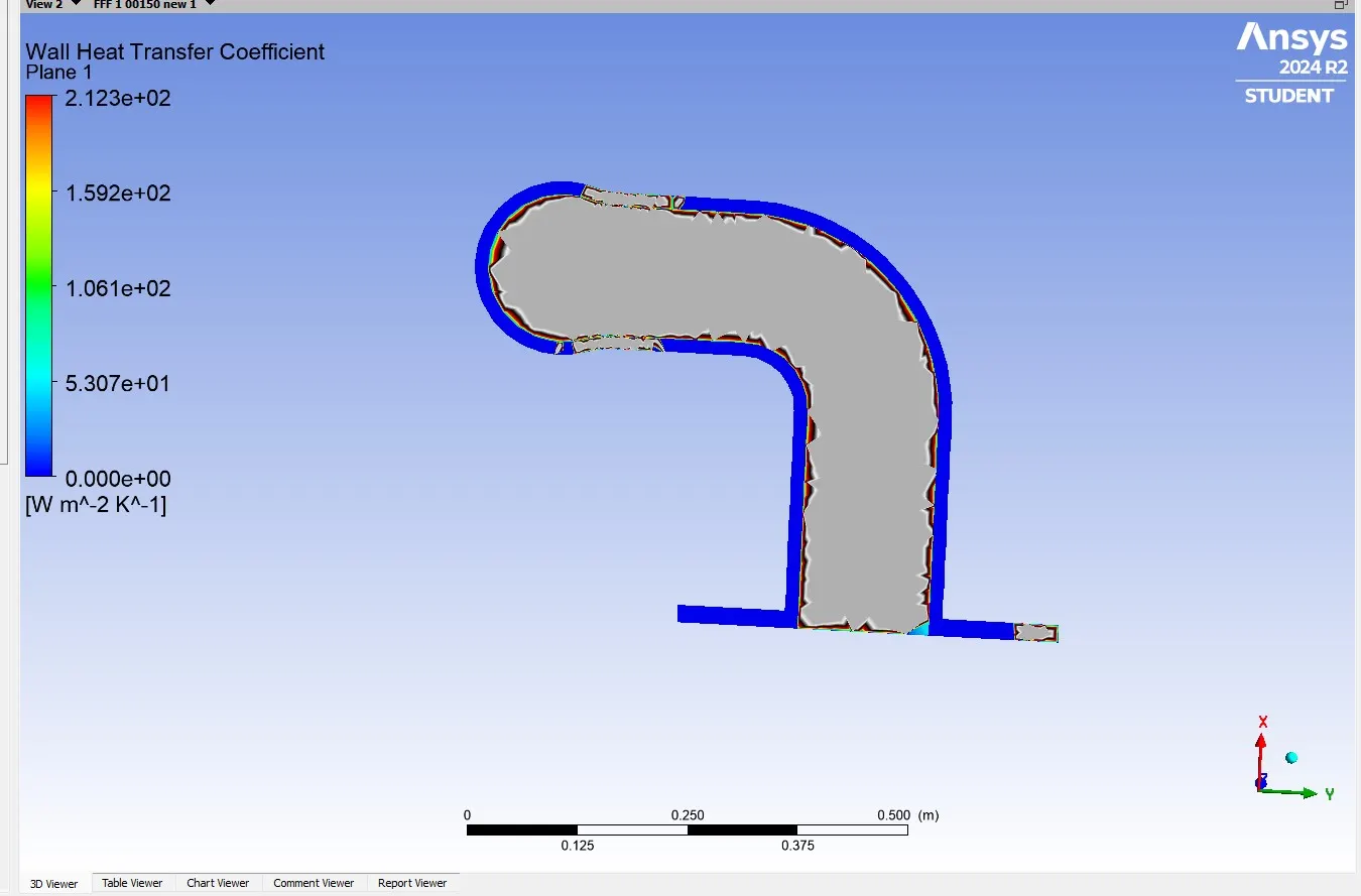
wall heat transfer coefficient on the internal solid surface contour:-

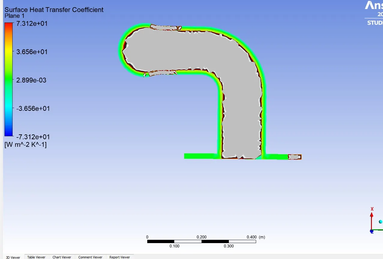
Surface heat transfer coefficient on the internal solid surface contour:-

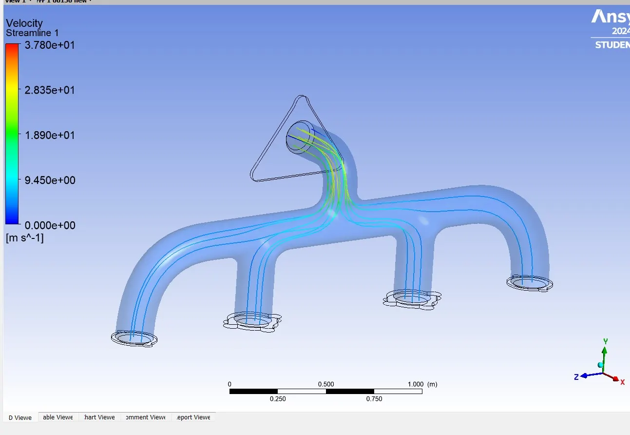
Velocity streamline plot:-

Velocity:-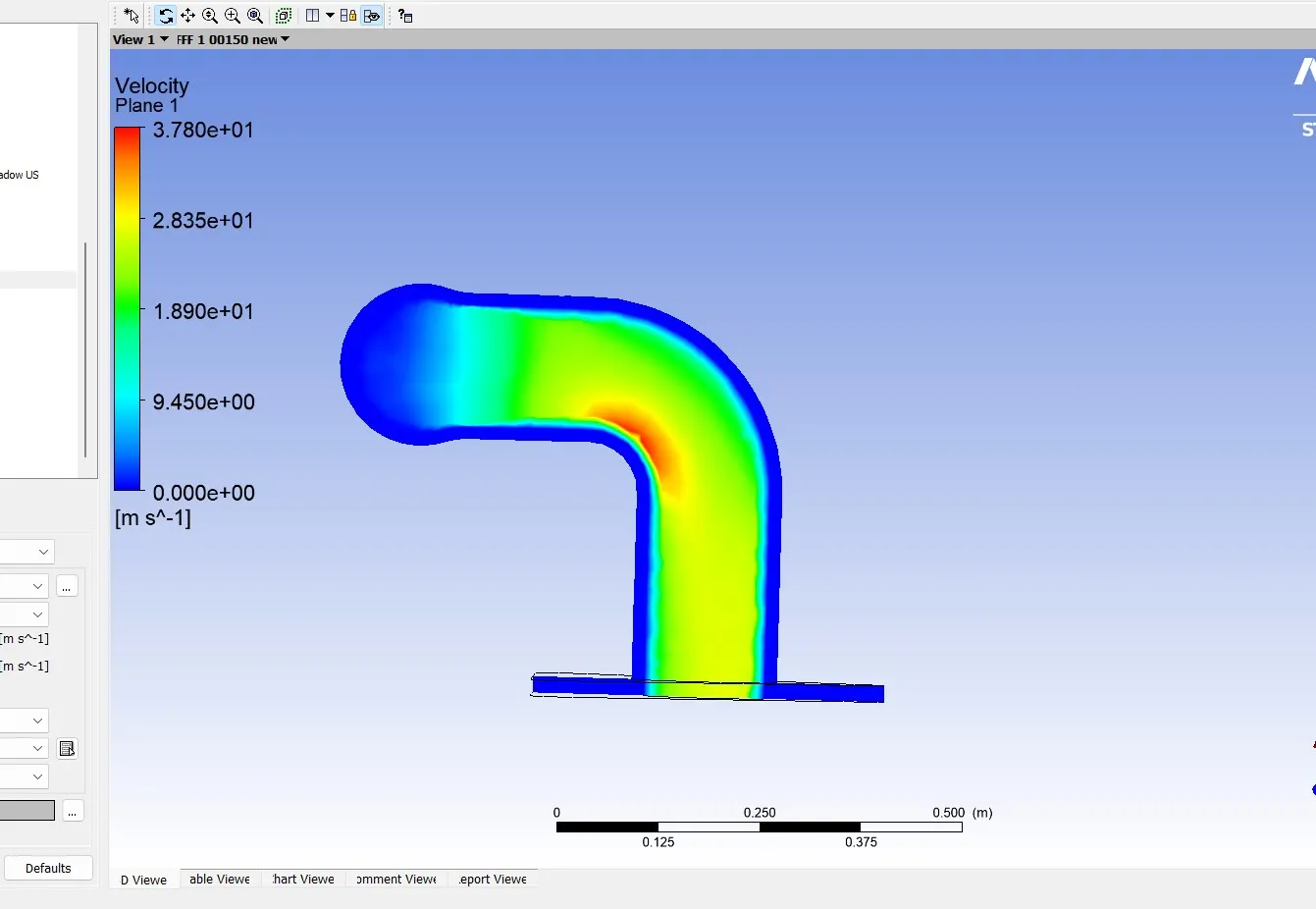

Temperature contour:-

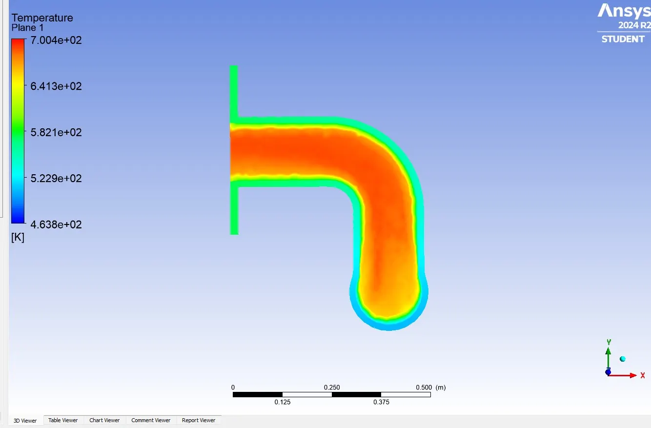
Refined mesh:-

The geometry is the same as the baseline simulation.

Meshing:-

Here we added one more name selection for the creation of an inflation layer. The inflation layer boundary is the outermost layer of the fluid volume which is selected by hiding the solid surface,

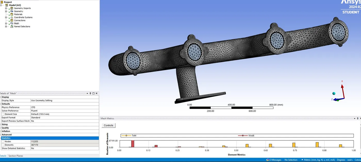
The inflation layer are calculated for the y+ value of 1 using an opensource boundary layer calculator.

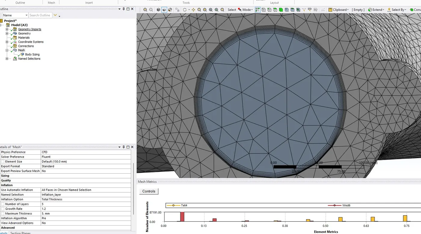
The mesh quality checked.

Setup and solution:-

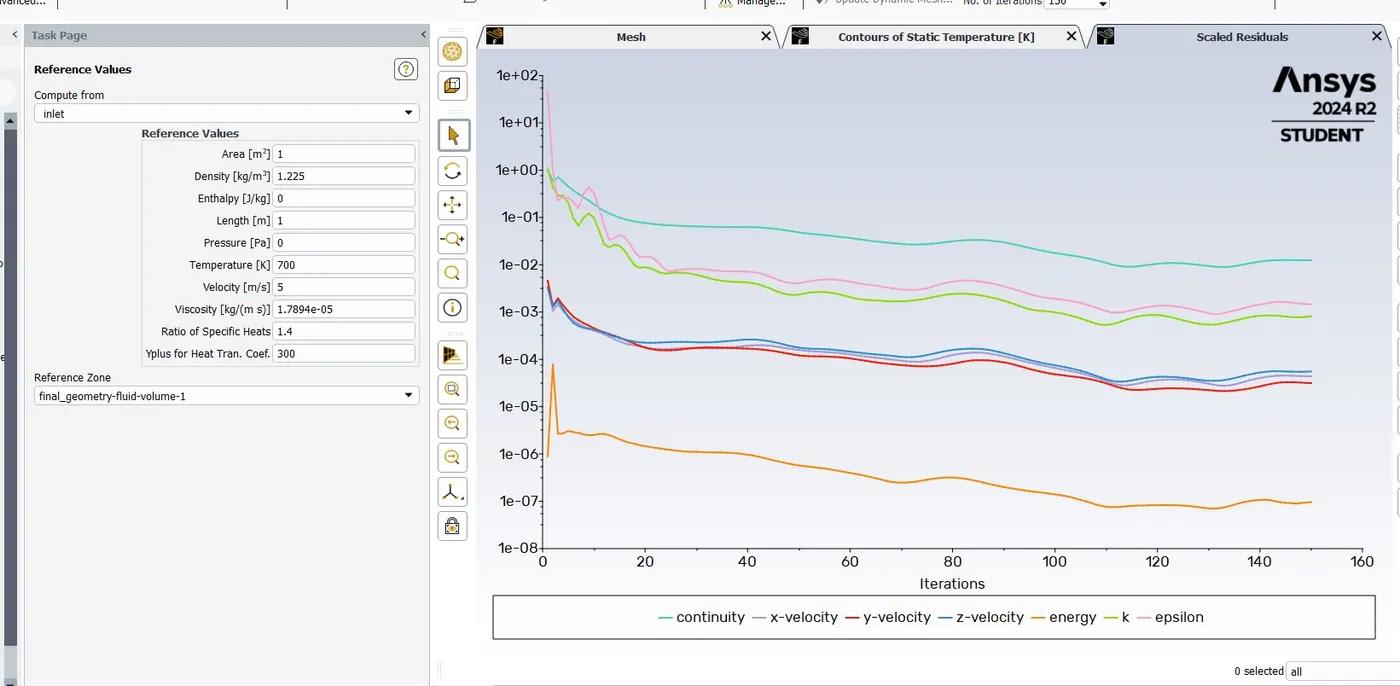
The k-epsilon turbulence model is used here,

Results:-

Residual plot:-

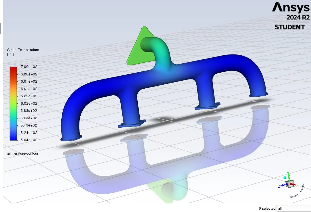
Temperature contour:-

Surface heat transfer coefficient on the internal solid surface plot:-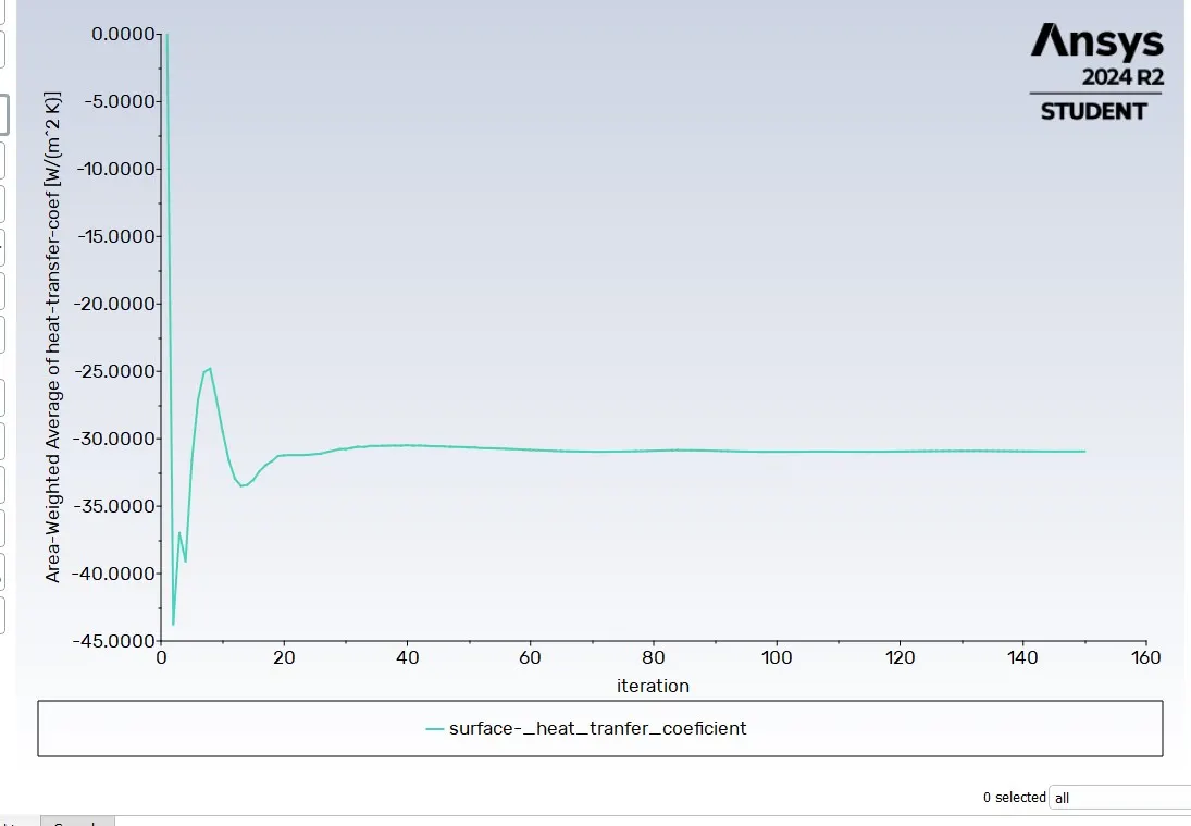

The outer surface heat transfer coefficient is also calculated

Surface heat transfer coefficient on the internal solid surface contour:-

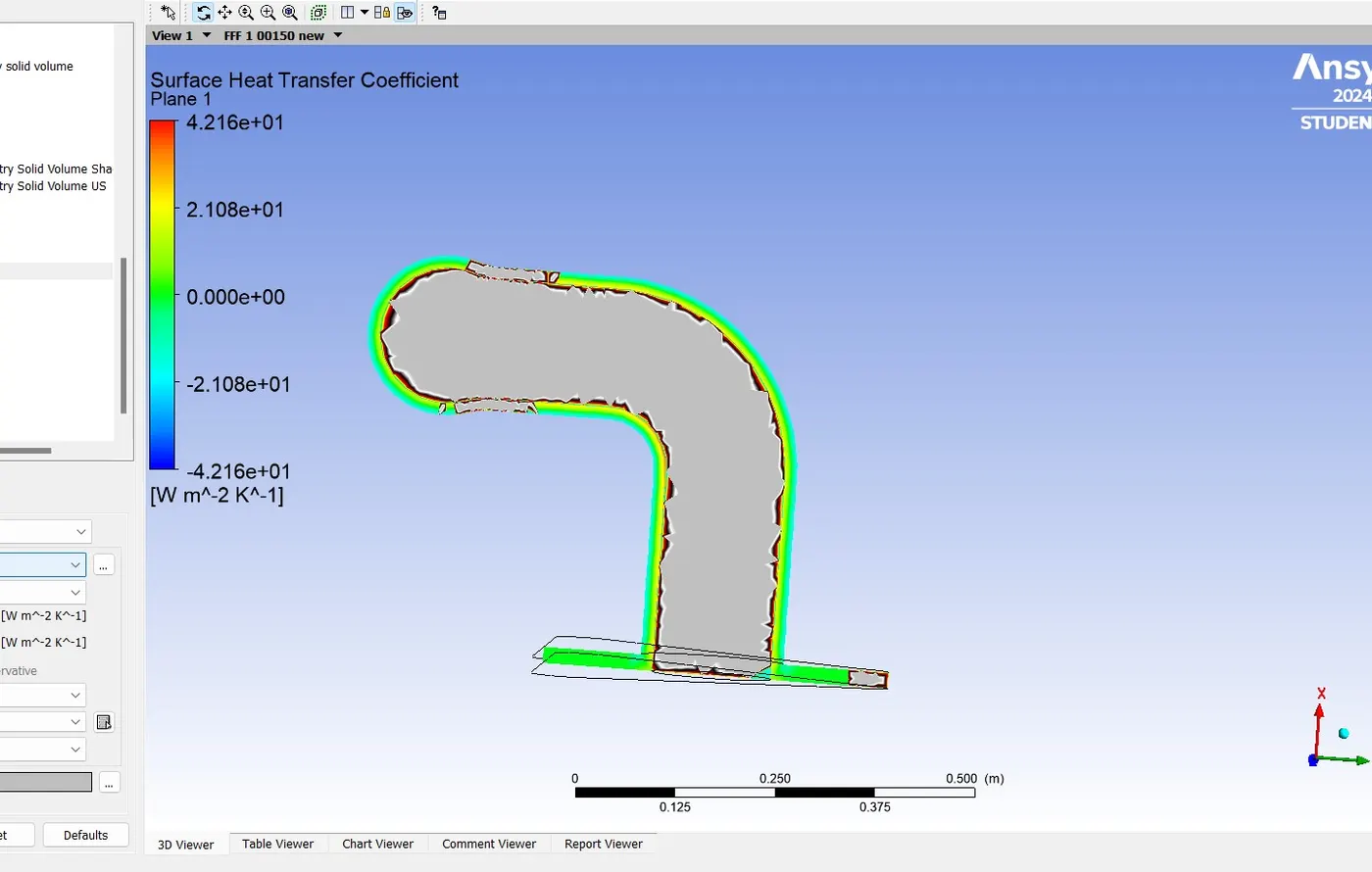
wall heat transfer coefficient on the internal solid surface contour:-

Velocity streamline plot:-

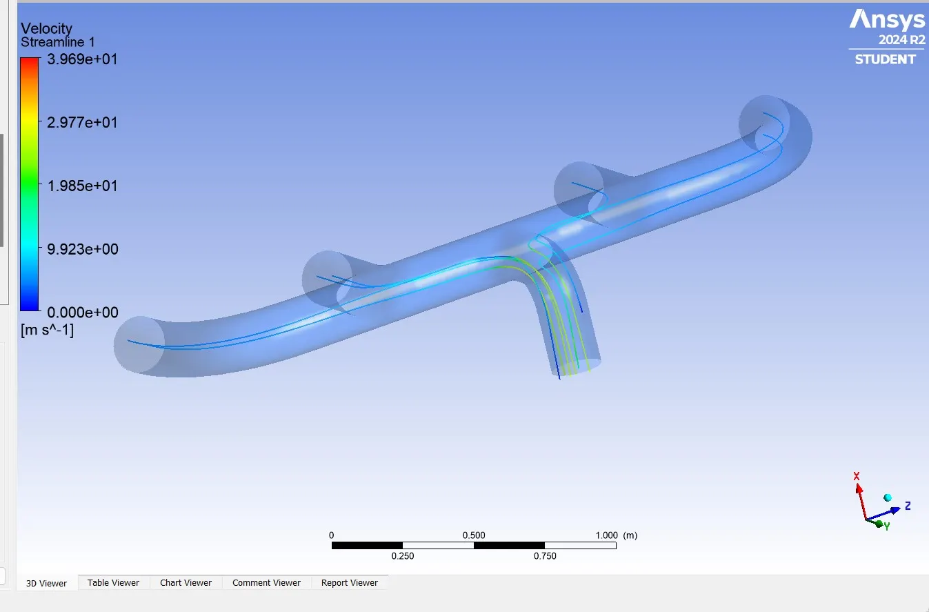
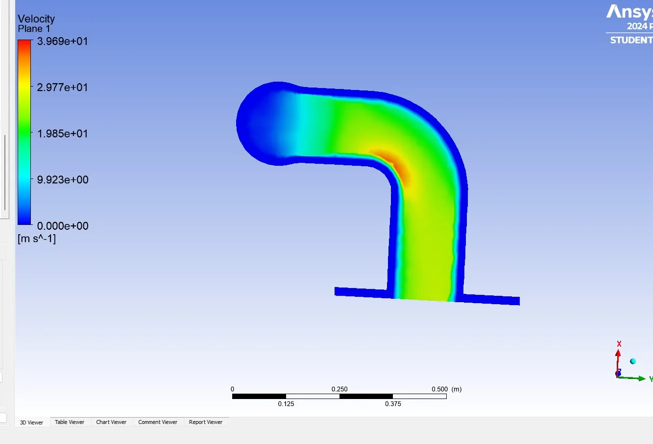
Velocity:-

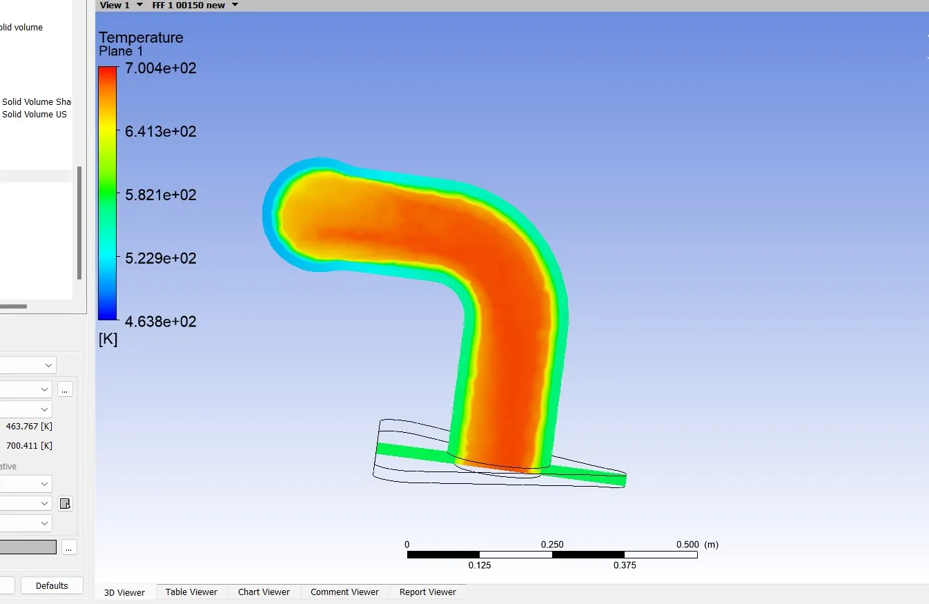
Temperature contour:-

Refined mesh(k-omega):-

Results:-K-omega turbulence model is used here

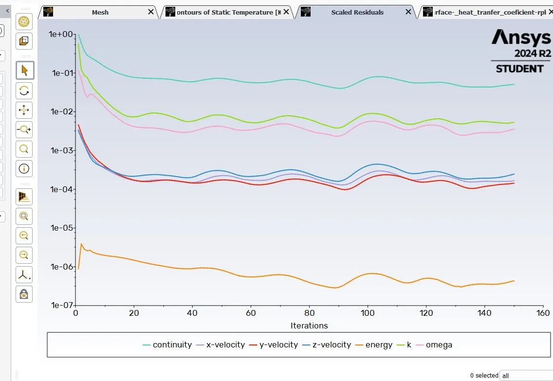
Residual plot:-

Temperature Contour:-

Surface heat transfer coefficient on the internal solid surface plot:-

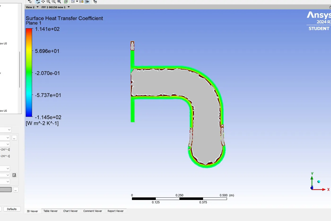
Surface heat transfer coefficient on the internal solid surface contour:-

wall heat transfer coefficient on the internal solid surface contour:-

Velocity streamline plot:-

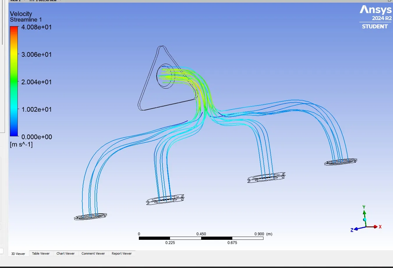
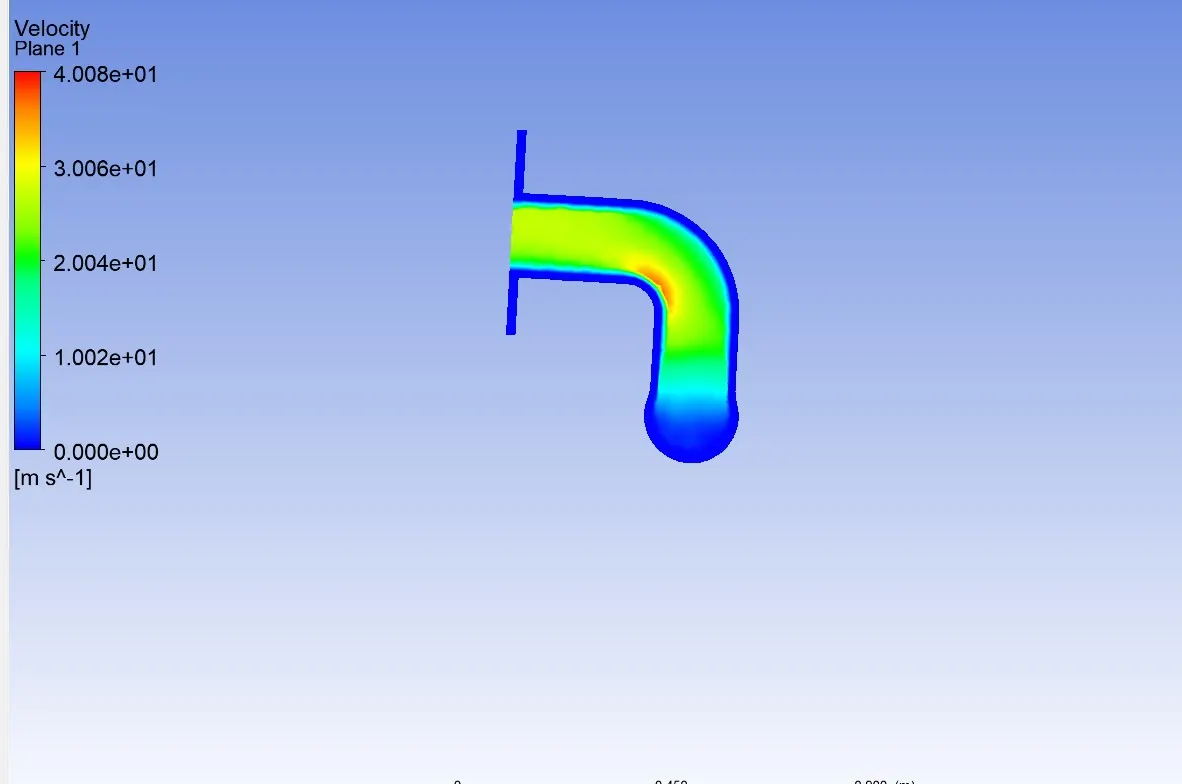
Velocity:-

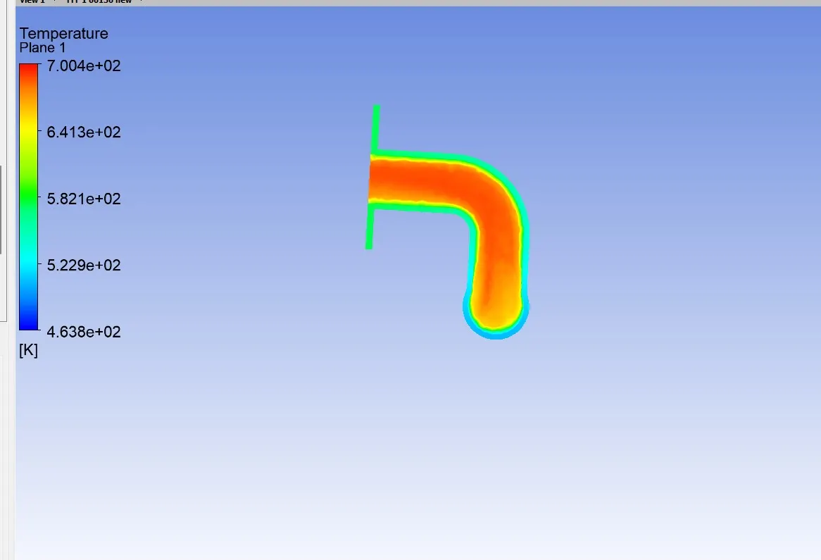
Temperature contour:-

Observation:-

As the hot air from the four inlets is made to pass through a single outlet pipe a high temperature is observed at the outlet.

The velocity is higher at the outlet region than at the at the inlet region. All the air from four inlets needed to exit the system through a single outlet, so due to mass conservation the velocity is high at the outlet.at the bend position of outlet, we can observe the highest velocity region.

The baseline simulation inner surface value was negative which is not good result, then we fixed after proper refinement of the mesh. Due to the high velocity outlet region, the Reynolds number is high at that region which means high heat transfer coefficient is also high at outlet.

The more heat is transferred between fluid and solid volume at the outlet region. The highest heat transfer coefficient is observed at the bend where velocity is the highest.

Heat transfer coefficient at the internal solid surface:-

Case name: Cell count: Numerical model: Surface heat transfer coefficient(inner surface)

Base line mesh 139386 K-epsilon -21.817617

Refined mesh 367170 K-epsilon 30.934953

Refined mesh 367170 K-omega 28.526289

The K-omega model gave the most accurate result of all and the k-omega model is recommended for flow near walls and for flows away from walls k-epsilon model is recommended.

Conclusion:-

The CHT analysis is explained briefly with its application and the simulation is performed successfully on the exhaust port. The y+ value of 1 was maintained for the refined mesh cases which increased the accuracy of the result and the best turbulence model suited for this problem was found to be the k-omega model. The surface heat transfer coefficient on the internal solid surface was calculated and the temperature and the velocity contours were plotted appropriately. The accuracy of the heat transfer coefficient depends on selecting the suitable y+ value and the turbulence model.