Week 4 - CHT Analysis on Exhaust port

Aim: To perform CHT analysis on an exhaust port.

WHAT IS CONJUGAT HEAT TRANSFER?

The Conjugate Heat Transfer (CHT) analysis type allows for the simulation of heat transfer between solid and fluid domains by exchanging thermal energy at the interfaces between them. Typical applications of this analysis type exist as, but are not limited to, the simulation of heat exchangers, cooling of electronic equipment, and general-purpose cooling and heating systems.

Applications of CHT:

Effective Heat Transfer

Efficiently combining heat transfer in fluids and solids is the key to designing effective coolers, heaters, or heat exchangers.

The fluid usually plays the role of energy carrier on large distances. Forced convection is the most common way to achieve high heat transfer rate. In some applications, the performances are further improved by combining convection with phase change (for example liquid water to vapor phase change). Even so, solids are also needed, in particular to separate fluids in a heat exchanger so that fluids exchange energy without being mixed.

Energy Savings

Heat transfer in fluids and solids can also be combined to minimize heat losses in various devices. Because most gases (especially at low pressure) have small thermal conductivities, they can be used as thermal insulators… provided they are not in motion. In many situations, gas is preferred to other material due to its low weight. In any case, it is important to limit the heat transfer by convection, in particular by reducing the natural convection effects. Judicious positioning of walls and use of small cavities helps to control the natural convection. Applied at the micro scale, the principle leads to the insulation foam concept where tiny cavities of air (bubbles) are trapped in the foam material (e.g. polyurethane), which combines high insulation performances with light weight.

INITIAL SETUP ON SPACE CLAIM:

• The file is loaded into the space claim software.
• Upon loading, the contour is checked for extra edges. If present, they are to be deleted using the extra edges tool in the repair section.
• Now the fluid voulme is created by selecting the volume extract tool in the prepare section. The edges of the inlet and outlet are selected and then the volume is extracted.
• In order to enable the transfer of data from the fluid domian to the solid domain, we must ensure that share option is used which is situated in the workbench section.
• It must be ensured that shared topology is enabled. This is to ensure that the solid volume and the fluid volume share information.

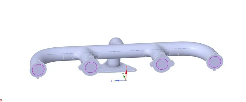
Exhaust Port

MESHING:

• Meshing is done as per requirement.
• For a baseline setup, we generally load the mesh with the default mesh settings and run the case.
• It is important to enable data sharing between the fluid domain and the solid domain in the space claim software itself. If not done, this may lead to improper data and readings. Also this leads to gaps in the meshing which intern lead to various misleading results.
• Below is the basic mesh:

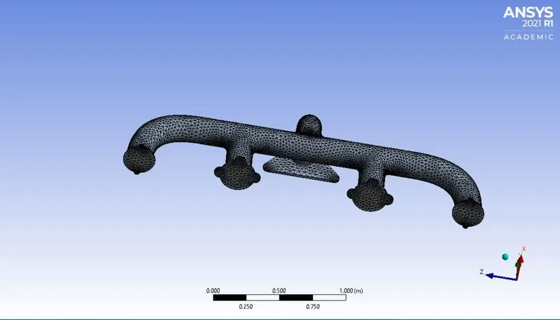
Meshing of the whole surface.

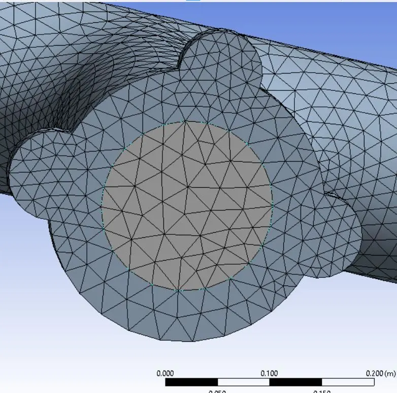
• Here we can observe that the meshing of the solid and the fluid volume is done as required. There are no gaps between the interface. This is to be ensured as we are running a conjugate heat transfer problem.
• In order to study the problem in detail, we add a few additions to the mesh, essentially decreasing the mesh size, adding inflation layers and various other options in order to observe the problem with precision and accuracy.
• The finer the mesh the accurate the result.
• Below is the refiend mesh:

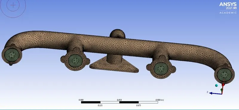
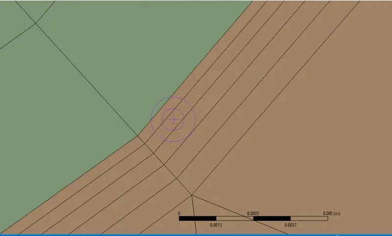
INFLATION LAYER

Basic Setup on Fluent:

• Once the revpious steps have been implemented,the fluent module is opened.
• Most of the required information such as values of density, velocity etc. are inputed in this module.
• The k-`epsilon` model was selected.
• Initially we setup the reference values as dipicted below:

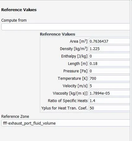
• Once we set the reference values, we also make sure to seup the matrial required and the boundary conditions.
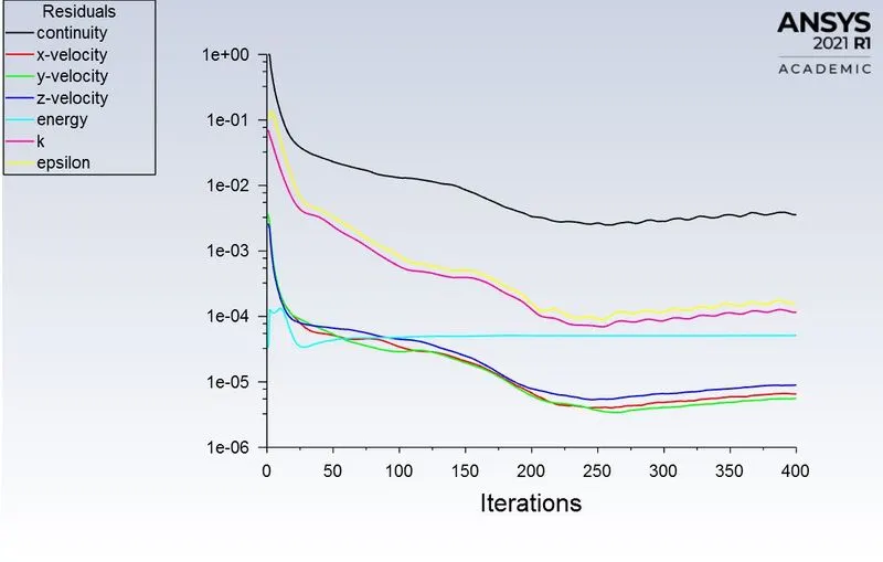
• Post this step we run the simulation for 400 step utilizing the SIMPLE method. This is done as this method is not computationally expensive and dosen't consume much time.

Baseline Setup:

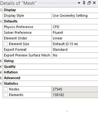
Mesh Size: 150 mm

No of elements:138182

Model: k-`epsilon`

Inlet Temperature: 700C

Inlet velocity: 5m/s

MESH:

Plots from Fluent:

Residuals:

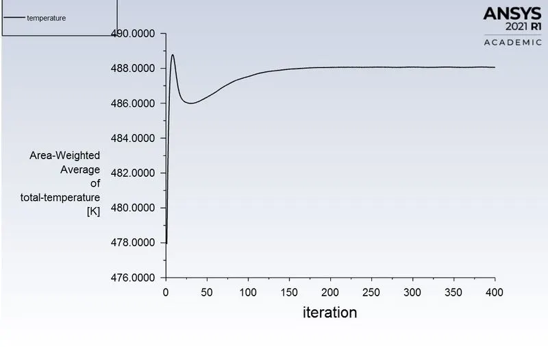
Temperature:

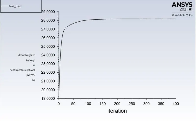
Heat trasfer coefficinet:

Post Processing plots:

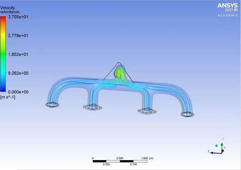
Stream Lines flow pattern for velocity:

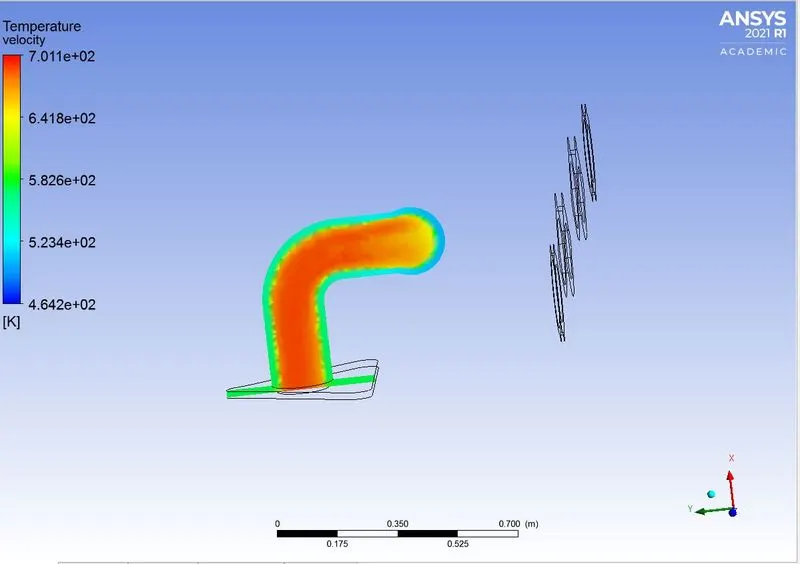
Temperature plane plot:

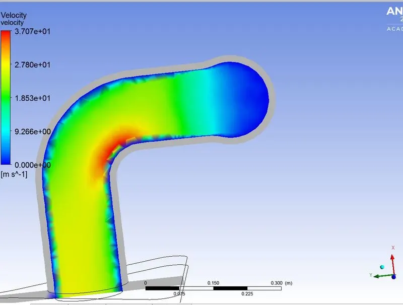
Velocity Plane Plot:

CASE 1:

Mesh Size: 150 mm

Body sizing element size: 15mm

No of elements: 312775

Model: k-`epsilon`

Inlet Temperature: 700C

Inlet velocity: 5m/s

Plots from Fluent:

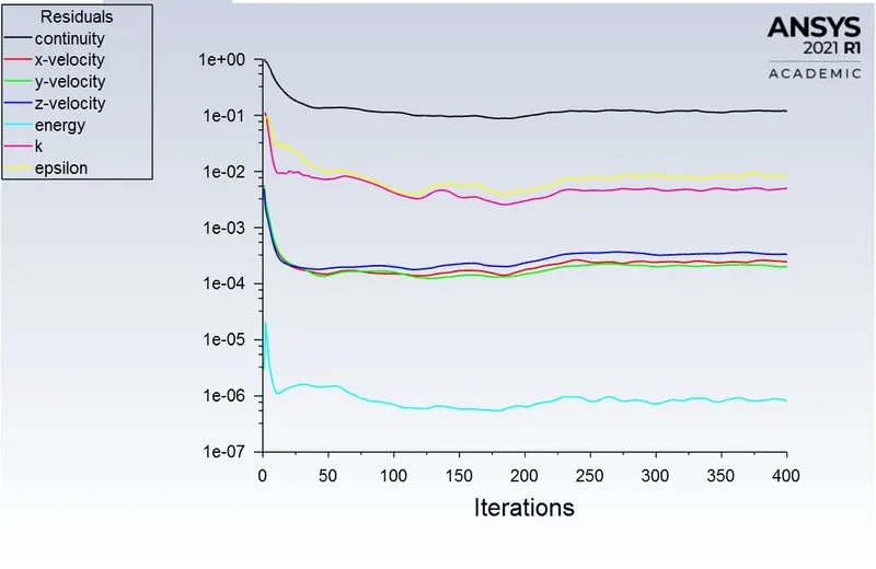
Residuals:

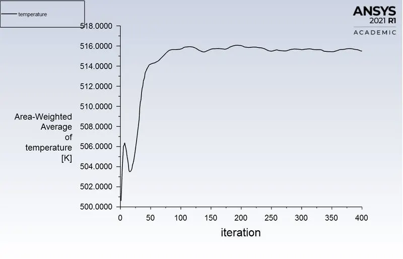
Temperature:

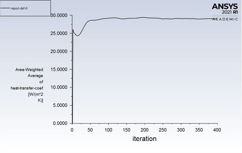
Heat trasfer coefficinet:

Post Processing plots:

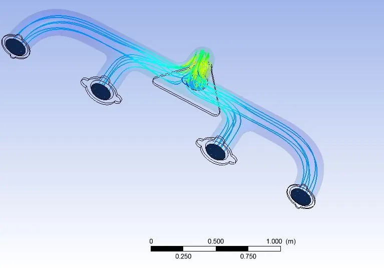
Stream Lines flow pattern for velocity:

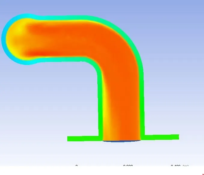
Temperature plane plot:

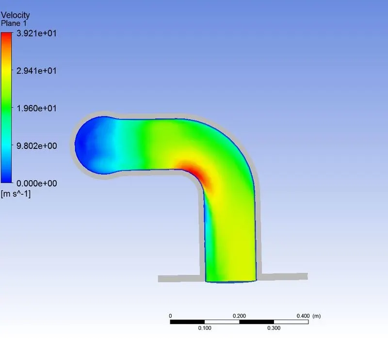
Velocity Plane Plot:

CASE 2:

Mesh Size: 150 mm

Body sizing element size: 15mm

No of elements: 312775

Model: k-`omega`

Inlet Temperature: 700C

Inlet velocity: 5m/s

Plots from Fluent:

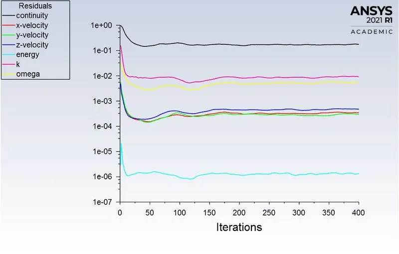
Residuals:

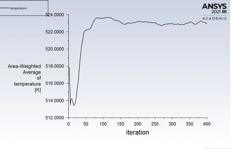
Temperature:

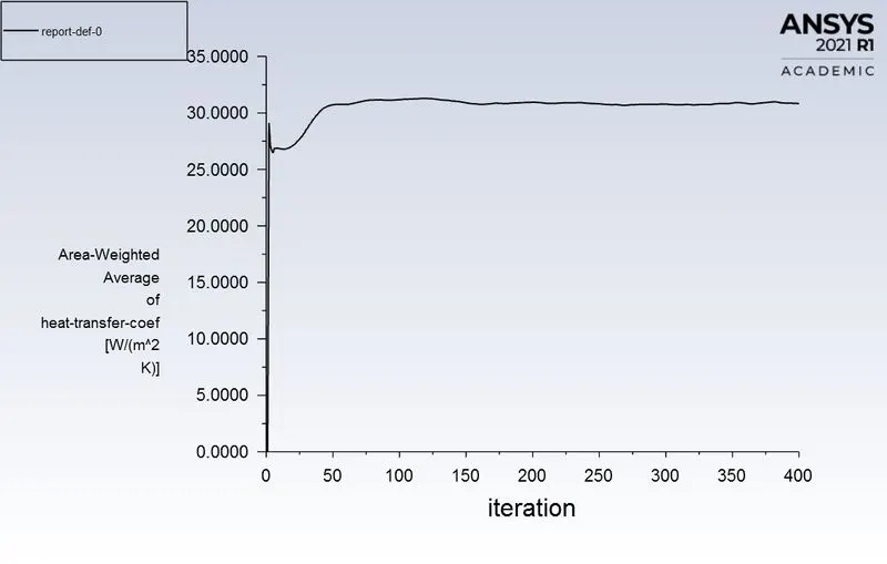
Heat trasfer coefficinet:

Post Processing plots:

Stream Lines flow pattern for velocity:

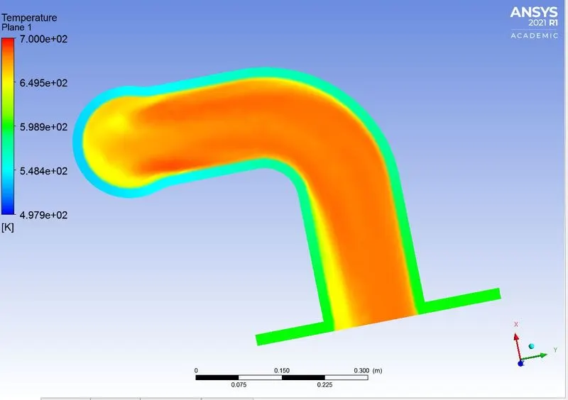
Temperature plane plot:

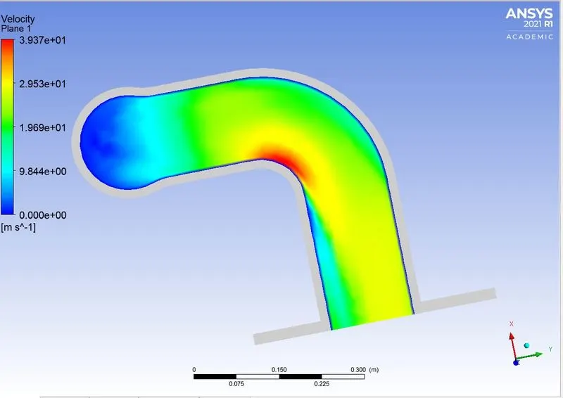
Velocity Plane Plot:

Inference:

• The baseline setup and the refiend setups have been run. The variations in results in each of them have been studied.
• The refiend version had been setup to a base mesh of 150mm and a body mesh of 50mm.
• In both case 1 and 2 the above configurations remain the same. However, the model used was different.
• Upon inspection, case 2 seemed to provide better results. This case employs the k-`omega` model which is cood with ow reynolds number simulations.
• Due to this, the k-`omega` model seemed to provide a stable solution compared to the former case.
• Also the temperature plots haven't shown much variation.
• When the number of elements are incresed, if can be observed that the solution is much more accurate. Due to computational and licence issues we cannot run this case for a smaller mesh size.
• In general, a smaller mesh size gives better results.

How would you verify if the HTC predictions from the simulations are right?

• In order to verify the HTC predictions from the simulation, a physical experiment is to be conducted. This can be mostly validated by creating a model of the exhaust and testing it applying similar conditions.
• A grid dependancy test can also be done to check if the predictions are correct.
• We could also validate this by the Dittus Boelter correlation:

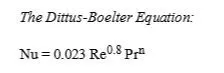
We know that,

Where h is the heat transfer coefficient between the fluid and the pipe wall, k is the thermal conductivity of the fluid, and D is the pipe diameter.

The above the the relation of reynolds number and velocity.

From the above equations, we can conclude that velocity is directly proportional to HTC. Since the plots for the velocity (PST) have been consistant iresspective of refinement, thus this simulation can be deemed accurate.

On what factors does the accuracy of the prediction depend on?

• Body Mesh Size
• Mesh quality
• Number of inflation layers and the sizing
• Geometry quality
• Type of physical model