Week 4 - CHT Analysis on Exhaust port

Aim: Performing conjugate heat transfer analysis on an exhaust manifold.

Objective:

• To familiarise with conjugate heat transfer (CHT) analysis.
• To set up solver for CHT analysis in a commercial CFD code (here, Ansys Fluent).
• To evaluate the heat transfer coefficient in the given heat transfer problem and validation of numerical results from a valid literary source.
• To set post-processing to obtain the required plots and contours and deduce the inference based on the results obtained.

Introduction:

The term conjugate heat transfer relates to the study of thermal interactions occurring at the interface between solid(s) and fluid(s) which includes convective (in fluids) and conductive (in solids as well as fluids) heat transfer where the convection can be either free (or natural) or forced. The analysis is governed by the set of equations that are conformal with the physics that separates the solid and fluid domains. The equations utilised are solid heat conduction (based on Fourier's law) and Navier-Stokes equations (Reynolds' Averaged (RANS) in case of turbulent flows). The applications of CHT analysis, although not limited, are profound in mechanical, aerospace, chemical, electronics, and nuclear engineering. Some typical areas of CHT analysis are:

• Heating, Ventilation, Air-conditioning and Refrigeration (HVAC&R)
• Heat exchangers and recuperators
• Boilers and its ancillaries
• Turbochargers
• Exhaust port
• Radiators
• Thermal management systems for electronic devices such as heat pipes for laptops, CPU cooling, battery thermal management systems (BTMS) for batteries

Workflow:

1. Preparing the geometry
2. Generate mesh for the geometry
3. Setting up the solver
4. Setting up the solution monitors
5. Post-processing to observe the results

Ansys Fluent:

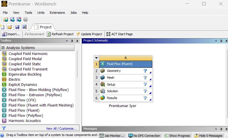In the Ansys workbench project window, Fluid Flow (Fluent) is dropped into the workspace.

Preparing the geometry:

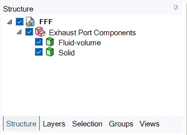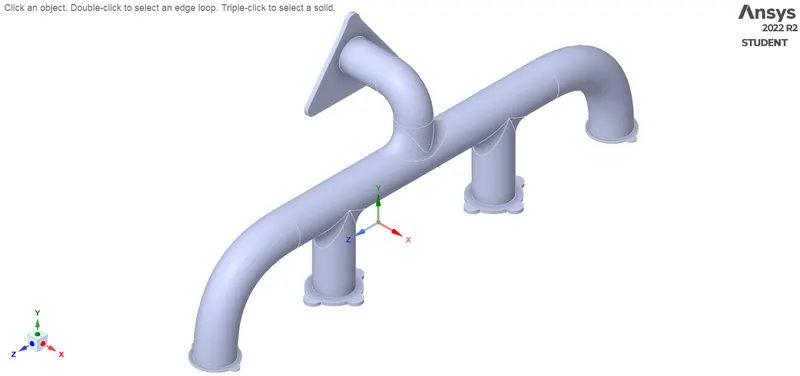
The computational domain, as shown (provided as a STEP file) is imported in SpaceClaim. The cleanup work begins with checking for any redundancies. The extra edges are carefully selected and removed and this can also be done by the extra edges option under the repair tab. Being an internal flow problem, the fluid flow volume is defined by means of the volume extract option available under the prepare tab. This is done by selecting the edges of the inlet(s) and outlet of the exhaust. Once, the volume is extracted, we have two components, fluid volume and the solid volume of the exhaust. The structure tree is modified in such a way that two components belong to the same component.

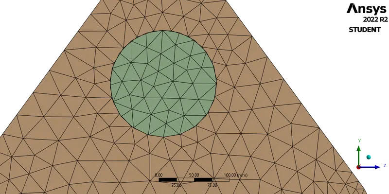A non-conformal mesh

However, when the meshing is done, it has some errors (the cell nodes are shifted in solid and fluid zones). This happens because the two regions are defined by their respective parts despite being from the same component and hence in SpaceClaim, these regions are selected and then the topology of these areas is shared from the properties drop don menu in the component structure tree. This ensures conformality in the generated mesh.

Generating mesh:

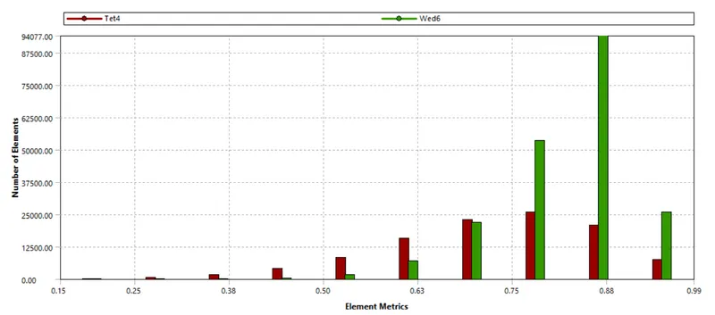
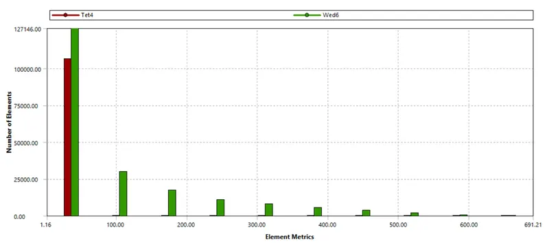
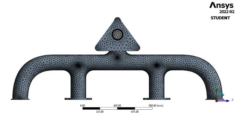
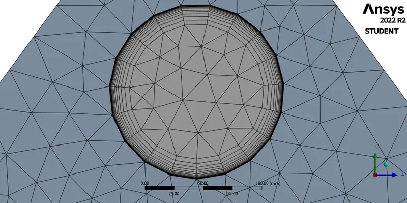
Meshing is the process, wherein the geometry is divided into smaller parts which are known as elements so that the iterative solver can solve the governing equations across the domain. In the meshing utility, a randomly provided element size is used which is consecutively revised (up to 150mm). Further, inflation layers are inserted and based on the y+ value the first cell height of 0.06mm with 17 layers having a growth rate of 1.3 was provided. This was done as the heat transfer is taking place at the interface of the walls and it is necessary to capture these effects. The generated mesh had 310024 elements. The mesh and the mesh metrics are as shown below:

Orthogonal Quality	Aspect Ratio

For implementing the boundary conditions, the "boundaries" must be clearly defined. To do so, the mesh utility itself has a tool; named selections. By selecting the respective faces and surfaces, the velocity inlet, the pressure outlet, convective walls (the outer walls exposed to the ambient), internal walls (which serve as the interface between the fluid and solid wall) and the fluid region (fluid volume).

Setting up the solver:

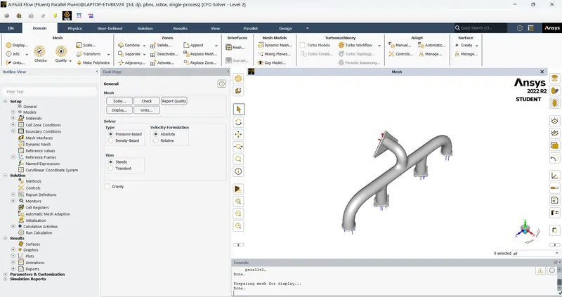An important part of a CFD simulation, the setup for solver is done to obtain the solution. Firstly, the units of important parameters are set to desired units (preferably SI units). In the models tab, in the viscous models, `k-omega` (shear stress transport - SST) is applied. The fluid zone contains air, and the default properties from the Fluent database are utilised. The boundary condition provided is summarised as:

Zone	Type	Value
Inlet	Velocity	`5m//s`
	Temperature	`700K`
Convective Walls	Heat Transfer Coefficient	`20W//m^2`
	Free Stream Temperature	`300K`
Outlet	Temperature	`300K`

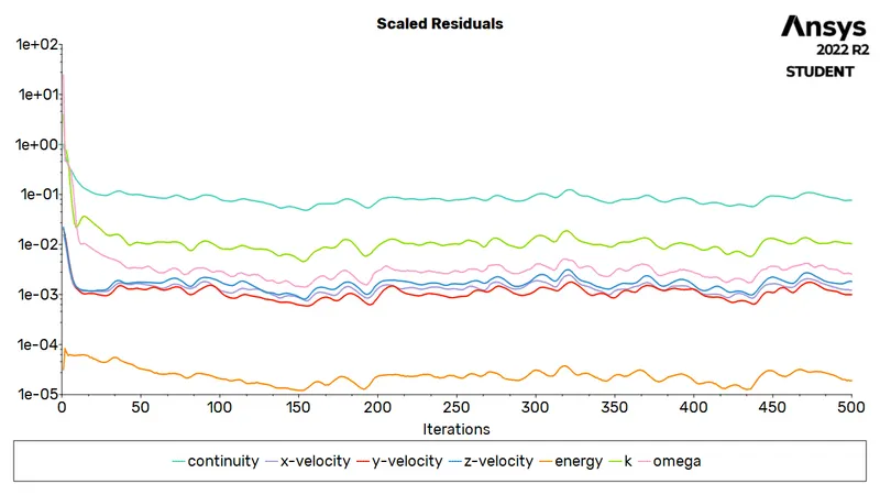
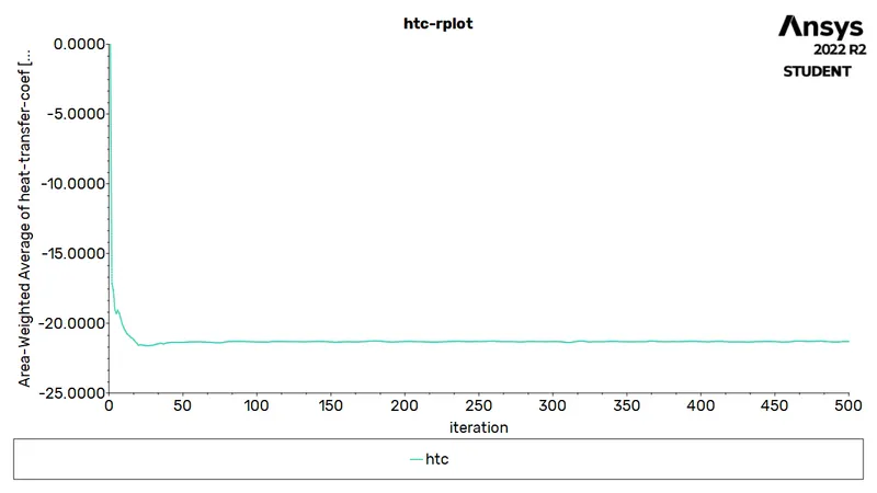
The pressure-velocity coupling is set to SIMPLE and the momentum and pressure are set to second-order discretisation. Report definitions are set to capture the coefficient of drag and lift over the car body surface. The corresponding plots along with the residual plots are saved. Hybrid initialization is used to initiate the problem, thereafter, 500 iterations are provided for the solver.

Post-processing (Results):

Scaled Residuals	Heat Transfer Coefficient (Area-weighted Average) 21.309124 `W//m^2 K`

	Plane1	Plane2
Pressure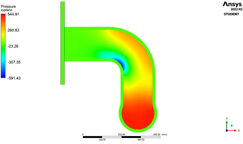
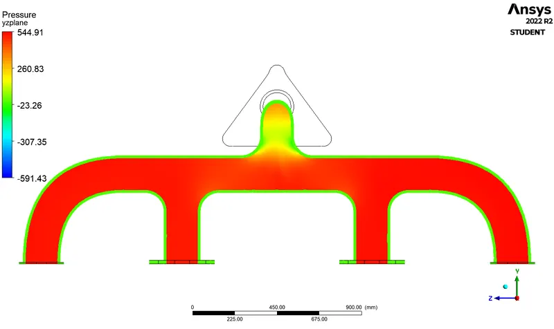Velocity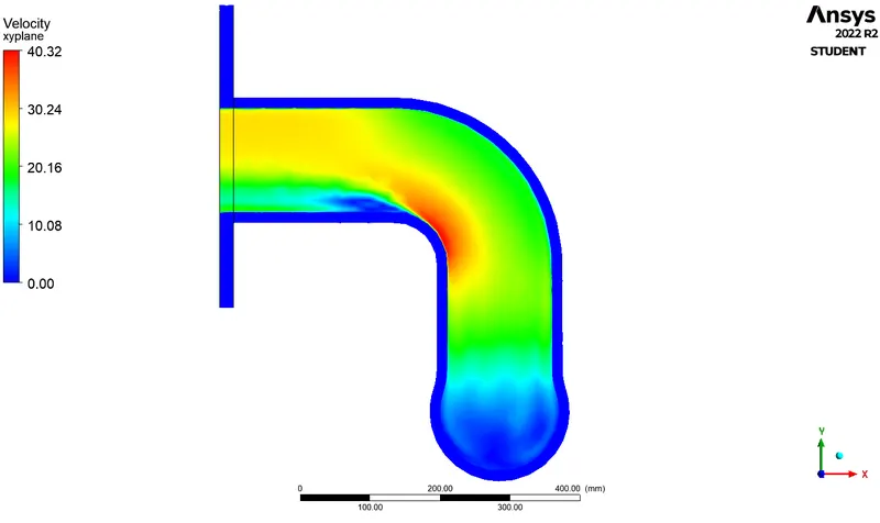
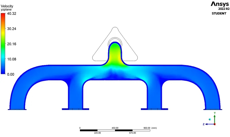Temperature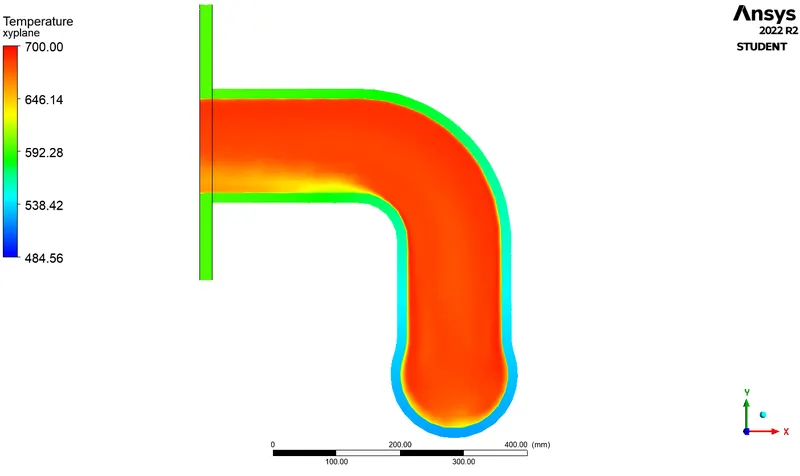
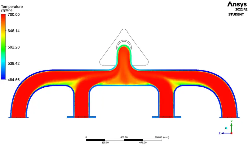Surface Heat Transfer Coefficient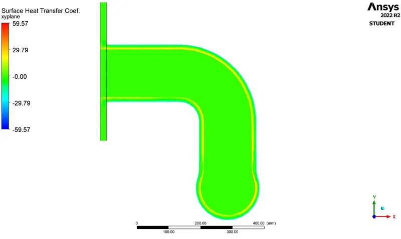

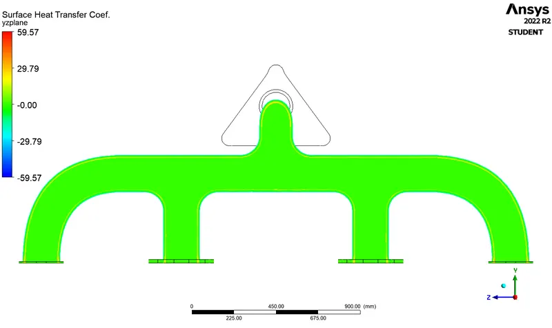	Contour
Streamline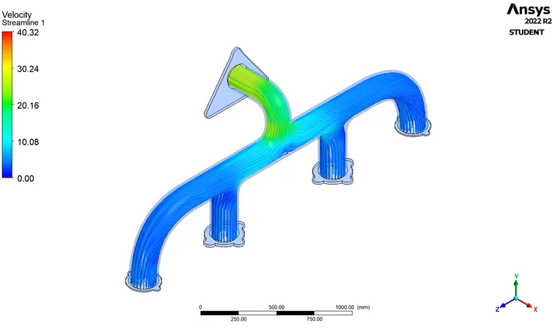
Surface Temperature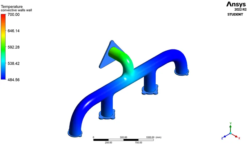
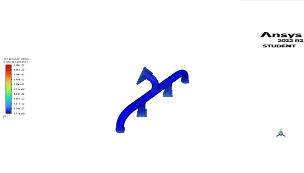
Surface Temperature Animation

The results can be verified from the analytical solution obtained from Dittus-Boelter equation:

`Nu_D = 0.023*(Re_D)^(4/5)*Pr^n` where `n` is `0.4` for heating and `0.3` for cooling

`Pr = (mu*C_p)/k`

`Re_D = (rho*v*D)/(mu)`

Also, `Nu_D = (h*D)/k`

Therefore, we have,

`Pr = (1006.43 xx 1.7894 xx 10^-5)/0.0242 = 0.744`

`Re_D = (1.225 xx 5 xx 166.1093 xx 10^-3)/(1.7894 xx 10^-5) = 56858.135`

`:. Nu_D = 0.023(56858.135)^(4/5)(0.744)^0.4 = 130.074`

Also, `Nu_D = (h*D)/k => h = (Nu_D*k)/D = 18.95 W//m^2 K`

Conclusion:

• As evident here from the temperature contour animation, there is a steady rise in the temperature of the walls of the exhaust. However, the rise is much greater at the bends near the exit. The reason behind this can be understood by simple enthalpy balance of the exhaust. At inlets, the hot fluid enters into the exhaust (and there are four inlets) and exits from the outlet. Hence,
  `dot(m_1)*h_1 + dot(m_2)*h_2 + dot(m_3)*h_3 + dot(m_4)*h_4 = dot(m_(out))*h_(out)` and
  `dot(m_1) + dot(m_2) + dot(m_3) + dot(m_4) = dot(m_(out))`
  
• Therefore, as the mass is conserved, and therefore, the mass of hot air leaving the exhaust is the sum of mass entering it and consequently the enthalpy of gas at exit is higher. This enthalpy is the function of temperature and thereby, it has been observed that the temperature of exhaust port surface near the exit is higher. The same is observed in the temperature contour in the cut section view of the exhaust port.
• The heat transfer coefficient is directly proportional to the Reynolds number. Therefore, the factors that cause the Reynolds number would also increase the heat transfer coefficient. In this case, the important factor is the inlet velocity and the dimensions (diameter) of the inlets.
• The analytical and experimental heat transfer coefficient is well in coherence. And we say that the simulation model utilised is correct.
• The accuracy of prediction is strongly dependant on the mesh quality. For cases involving fluid flow (such as this one) an appropriate turbulence model has to be used in accordance with the y+ value. Apt y+ value helps in calculating total and first layer thickness for the inflation from the wall for the better capturing of effects near the wall, which is the Heat transfer coefficient in our case. Also, one needs to make sure that the topology of the components is shared to form a conformal mesh.
• The most important aspect in any numerical approach is GIGO (Garbage Input - Garbage Output). The outputs generated from the numerical methods (simulations) are as good as the inputs. If the inputs in themselves are erratic, so would be the outputs.

References:

• Introduction to GUI based CFD using Ansys Fluent - Course provided by Skill-Lync
• Ansys Inc.
• Volupe Engineering Software: y+ calculator
• Supporting Material: Comsol blog: Conjugate Heat Transfer
• Supporting Material: A-TO-Z GUIDE TO THERMODYNAMICS, HEAT & MASS TRANSFER, AND FLUIDS ENGINEERING
• Supporting Material: Application of Conjugate Heat Transfer Simulations for the Development of Ventilation and Cooling Systems for Large Hydro Generators
• Supporting Material: ASME: Specific Applications of Conjugate Heat Transfer Models
• Supporting Material: Fluid Mechanics - Frank M White
• Supporting Material: Heat Transfer - Y Cengel and A Ghajar