Week 4 - CHT Analysis on Exhaust port
Aim
Perform CHT Analysis on Exhaust Port.
- Give a brief description of why and where a CHT analysis is used.
- Maintain the y+ value according to the turbulence model and justify the results.
- Calculate the wall/surface heat transfer coefficient on the internal solid surface & show the velocity & temperature contours in appropriate areas.
- How would you verify if the HTC predictions from the simulations are right? On what factors does the accuracy of the prediction depend on?
Conjugate Heat Transfer(CHT):
The Conjugate Heat Transfer (CHT) analysis type allows for the simulation of heat transfer between solid and fluid domains by exchanging thermal energy at the interference between them. A typical application of this analysis type exists as but is not limited to the simulation of heat exchangers, cooling of electronic equipment, and general-purpose cooling and heating systems.
The contemporary conjugate convective heat transfer model was developed after computers came into wide use in order to substitute the empirical relations of proportionality of heat flux to temperature difference with heat transfer coefficient which was the only tool in theoretical heat convection since the times of Newton. This model based on a strictly mathematically stated problem describes the heat transfer between a body and fluid flowing over or inside it as a result of the interaction of two objects. The physical processes and solutions of the governing equations are considered separately for each object in two subdomains. Matching conditions for these solutions at the interface provide the distributions of temperature and heat flux along with the body flow interface, eliminating the need for a heat transfer coefficient.
Why CHT analysis is used:
- CFD and more specifically CHT analysis can accurately predict heat transfer by simultaneously solving all the relevant solid and flow field heat transfer processes, for e.g, conduction through solids, free and forced convection in the gases/fluids, and thermal radiation.
- The CHT approach has an advantage over Finite element thermal analysis in that wall heat transfer coefficients and their local variations on surfaces are directly calculated within the model rather than based on simplified empirical calculations. The CHT approach, therefore, has benefits for these applications where heat transfer is either non-uniform or difficult to calculate empirically.
Where is CHT analysis used:
Starting from simple examples in the 1960s, the CHT method has become a more powerful tool for modeling and investigating natural phenomenon and engineering systems in different areas ranging from aerospace and nuclear reactions to thermal goods treatment and food processing, from the complex procedure in medicine to atmosphere/ocean thermal interaction in metrology, and from relatively simple units to multistage, nonlinear processes.
Applications:
- Internal Combustion Engines
- Electromobility
- Pumps and Compressor
- After-treatment Systems
CASE 1: Baseline Simulation
Element size: 0.15m
No. of Element: 1,35,711
Viscous Model: K-epsilon
Inlet Velocity: 5m/s
Inlet Temperature: 700K
Heat transfer coefficient: 20 W/m2K
Geometry Set-up:
- Load the model into SpaceClaim and change the units into meters.
- Remove the duplicate edges in the model.
- Then extract the fluid volume and give the name inner volume as fluid and outer volume as solid and remove the empty component.
- Enable the shared topology of the main component so that the mesh and physics information can be shared conformal mesh can be achieved.
- Lastly, to achieve conjugate heat transfer between the fluid and wall we have to choose share prep under the workbench tool so that heat transfer is captured throughout the wall from inlet to outlet.
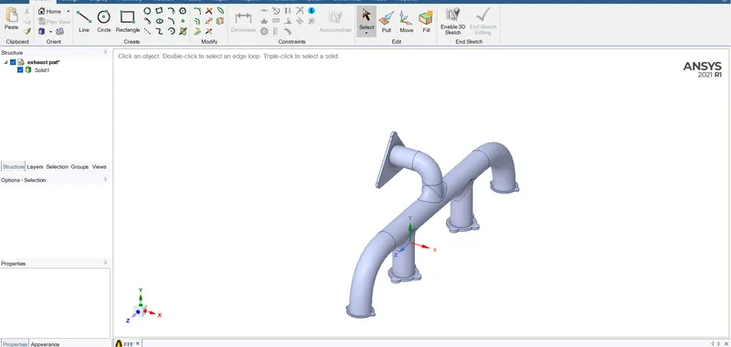
Opening geometry in Spaceclaim

Changing the unit
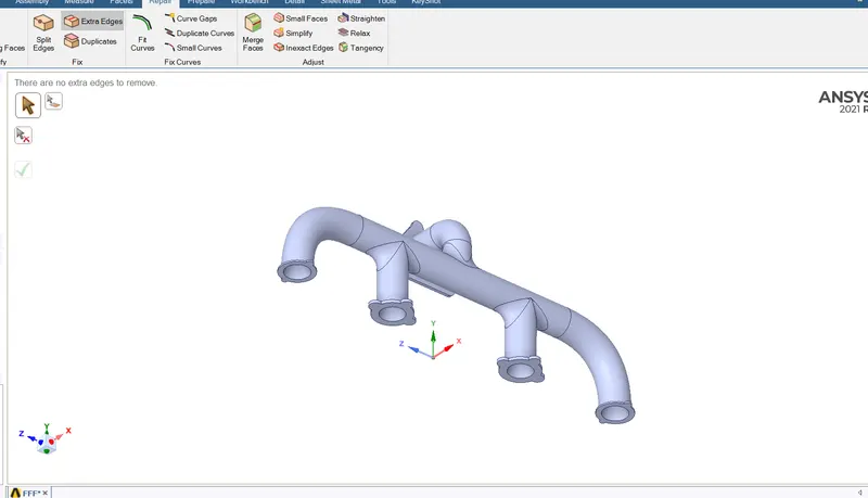
Checking for any extra edges present
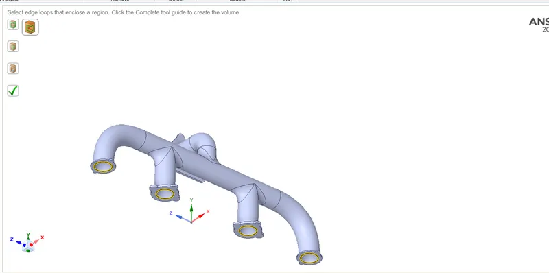
Doing Volume extraction

DOING SHARE TOPOLOGY
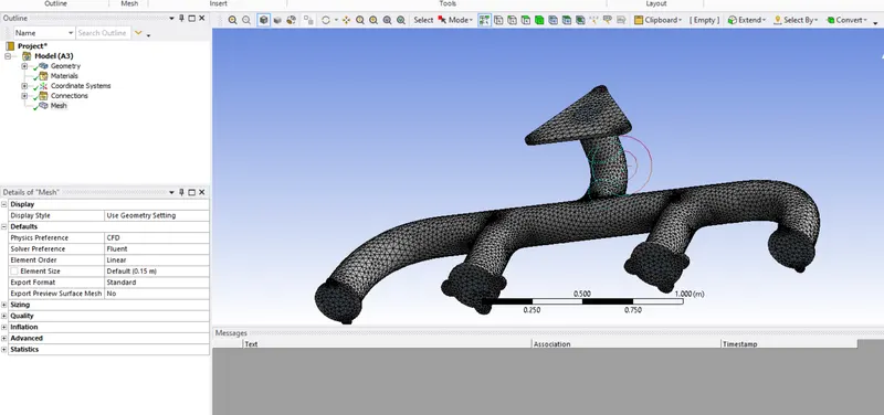
Done Default Meshing
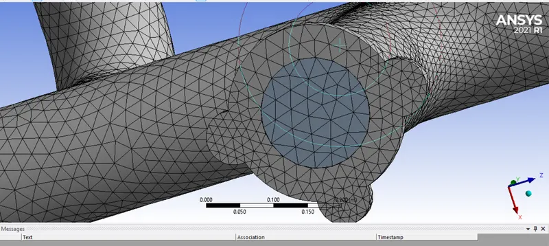
From this it is clear that the interface between solid and fluid is matching perfectly
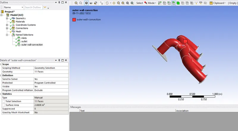
Given naming to parts
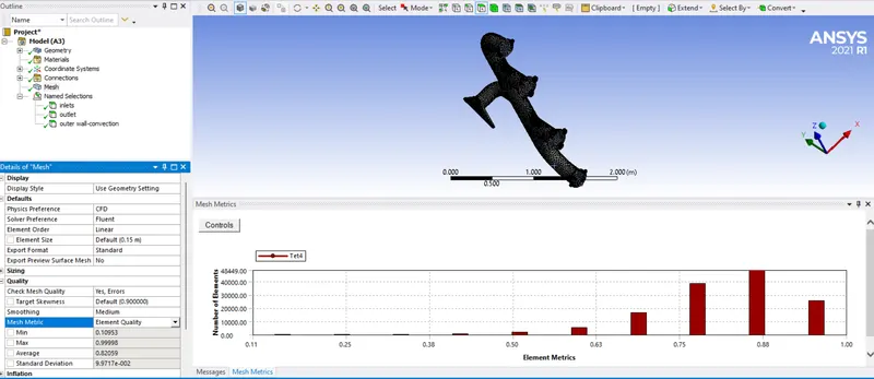
Checking mesh quality

Opening Setup window
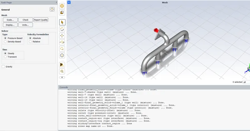
Using pressure -based solver and steady state analysis
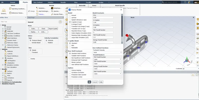
Using K-Epsilon turbulence model with standard wall function
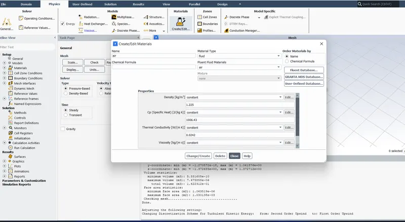
Adding material
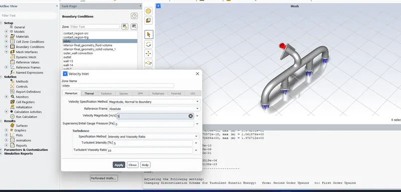
Giving inlet boundary conditions
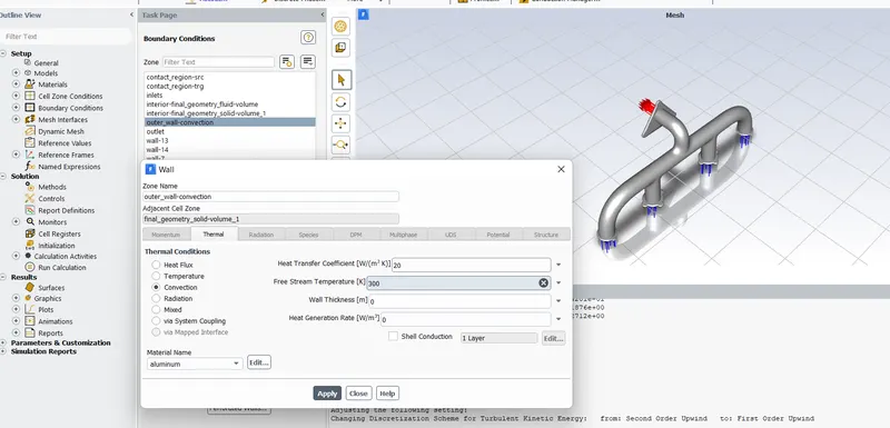
Giving value for convective heat transfer coefficient
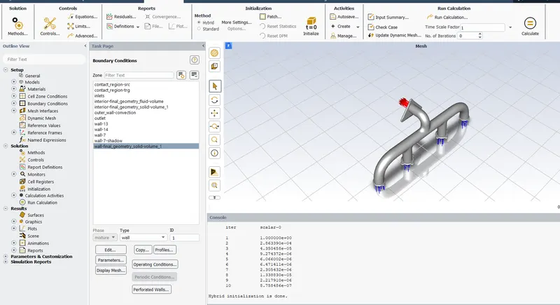
Hybrid Initialization done
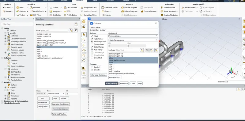
Setting temperaure contour
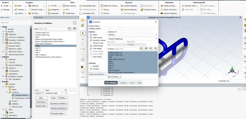
Setting velocity contour
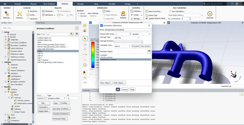
Setting temperature animation
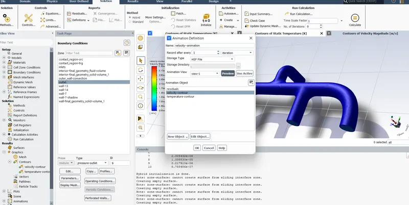
Setting velocity animation
RESULTS AND DISCUSSIONS:
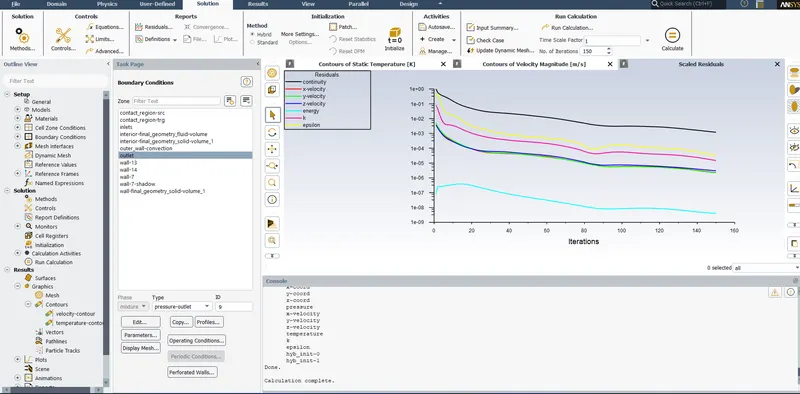
Showing Residuals
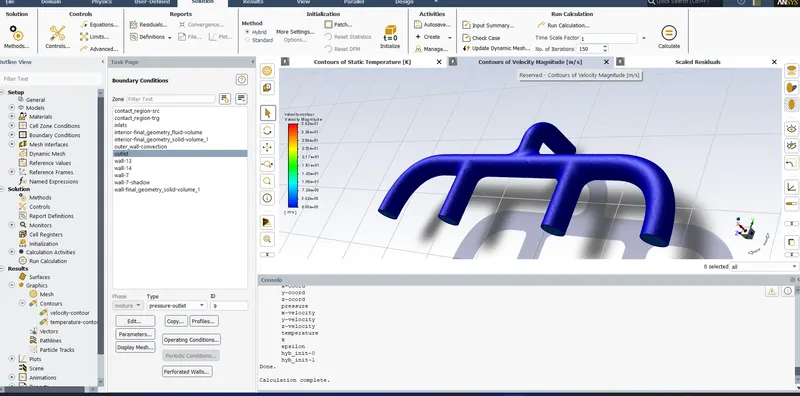
Showing velocity contour
It is clear that velocity is almost same everywhere
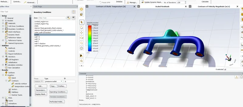
Showing temperature contour
Here we can see the variation of temeperature. From this it is clear that temperature is around 400K on the walls near to the inlet ports and temperature is around 600K on the wallls near to the outlet.This is beacuse of the variation in the velocity.Here volume flow rate is constant and area is decreasing towards outlet due to one number of outlet and which is compensated by increasing the velocity.As a result the convective heat transfer coefficient is more and which leads to more heat transfer from the insidefluid to the outer material and therefore temperature is more at the walls near to the outlet and bend.
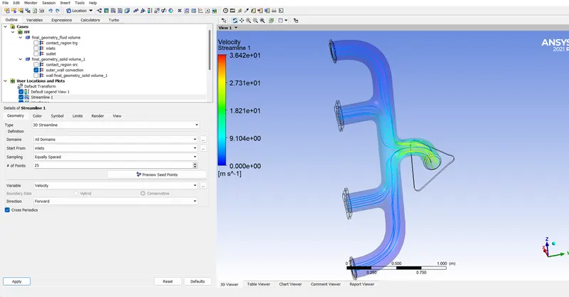
Showing velocity stream lines
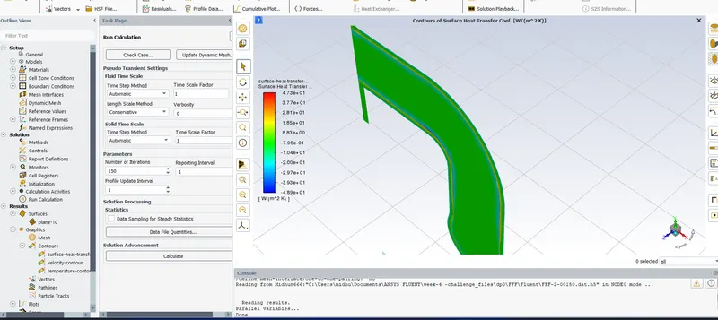
Showing contours of surface heat transfer coefficient
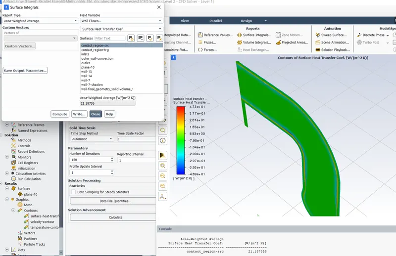
Showing value of surface heat transfer coefficient
From this it is clear that the value of Surface heat transfer coefficient is 21.18735W/m2K
CASE 2: Refined Simulation
Element size: 0.010m
No. of Element: 5,38,671
Viscous Model: K-epsilon
Inlet Velocity: 5m/s
Inlet Temperature: 700K
Heat transfer coefficient: 20 W/m2K
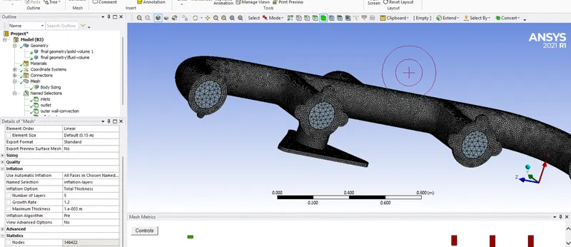
Showing refined mesh
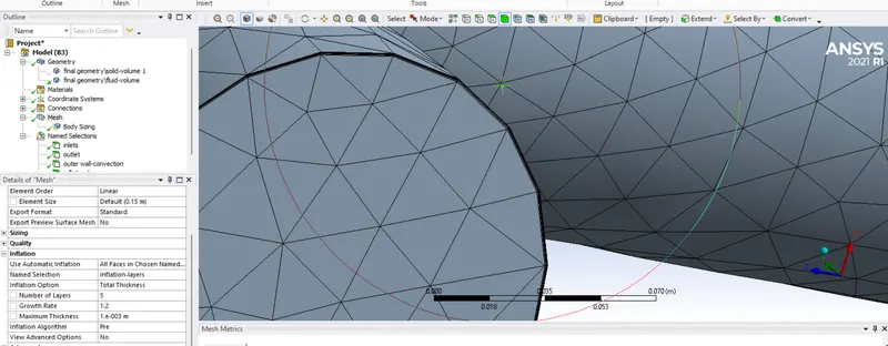
Inflation layers added at the interface
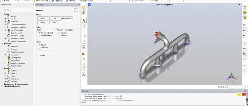
Mesh checking done
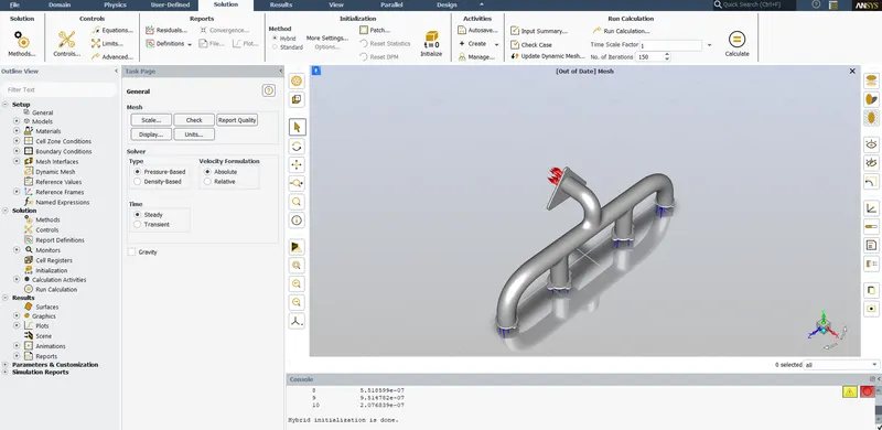
Hybrid Initialization done
RESULTS AND DISCUSSIONS:
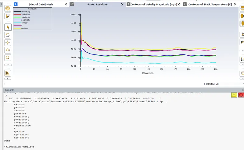
Showing residuals
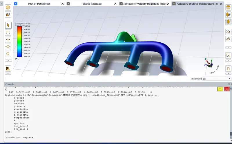
Contour of static temperature
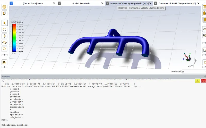
Contour of velocity
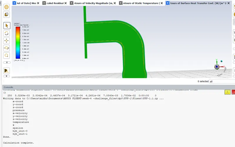
Contour of surface heat transfer coefficient
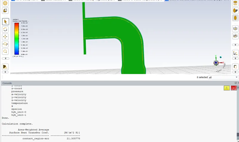
Showing the value of surface heat transfer coefficient.
From this it is clear that here the surface heat transfer coefficient is 21.30577W/m2K.
CASE 3: Refined Simulation
Element size: 0.01m
No. of Element: 5,38,671
Viscous Model: K-Omega(SST Model)
Inlet Velocity: 5m/s
Inlet Temperature: 700K
Heat transfer coefficient: 20 W/m2K
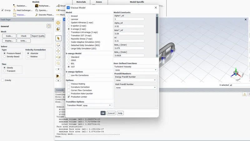
Using K-Omega SST Model
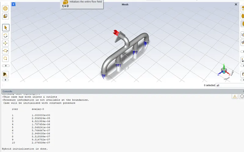
Hybrid Initialization done
RESULTS AND DISCUSSIONS:
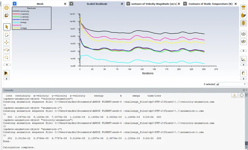
Showing residuals
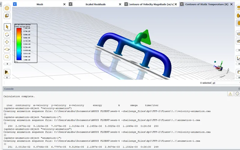
Contours of temperature
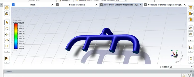
Contours of velocity
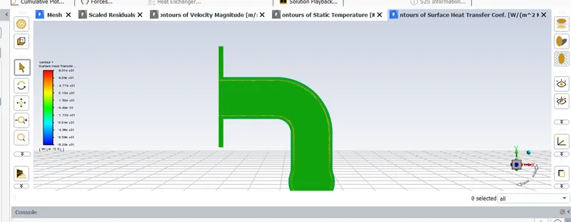
Contours of surface heat transfer coefficient
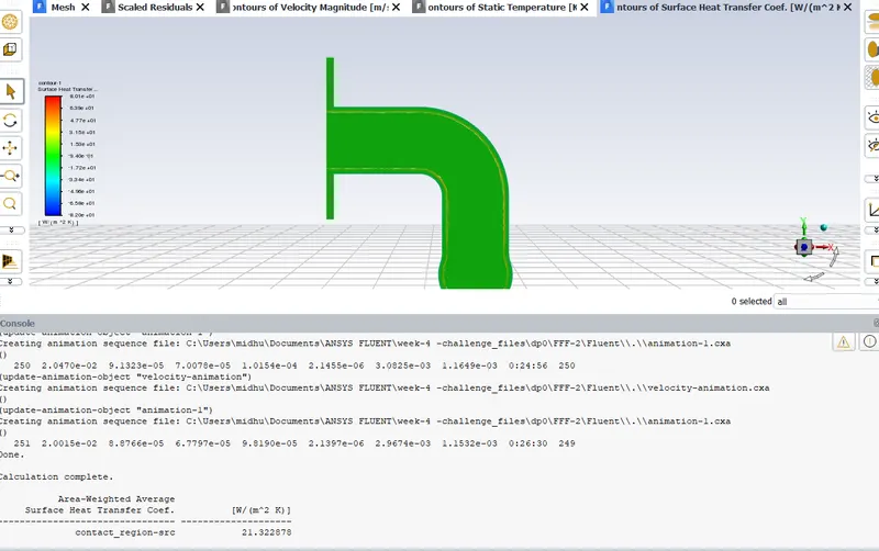
Value of surface heat transfer coefficient is 21.322878W/m2K
COMPARISION OF DIFFRENT CASES:
| CASES | TURBULENCE MODEL | NO OF CELLS | SURFACE HEAT TRANSFER COEFFICIENT |
| (1) | K-Epsilon | 1,35,711 | 21.18735 |
| (2) | K-Epsilon Refined | 5,38,671 | 21.3057 |
| (3) | K-Omega SST | 5,38,671 | 21.322878 |
How would you verify if the HTC predictions from the simulations are right? On what factors does the accuracy of the prediction depend on?
According to Bernoulli's mass conservation principle mass is conserved in our model which is clearly explained below;
Let us assume the flow rate from each inlet as Q1, Q2, Q3, Q4 respectively, and Q5 be the flow rate from the exhaust manifold.
As mass is neither created nor destroyed, mass flow rates are also balanced as below;
Q1+Q2+Q3+Q4=Q5 ...........(1)
we have Q= ρ⋅A⋅Vρ⋅A⋅V ...........(2)
Now equation 1 becomes
A1V1+A2V2+A3V3+A4V4=A5*V5
As it is an incompressible flow to compensate for mass flow, velocity is increased. and the overall mass flow rate is conserved.
As velocities are high, the Reynolds number at the outlet manifold will be high.
Nu=f(Re,Pr) for forced convection application.
Nu= hD/k
from above formula Nudirectly∝directly∝ Re. Hence Nu∝∝h, therefore, Re∝∝h.
From our simulation, we have observed velocities are high at bend section of outlet manifold hence higher Reynolds number which was at high heat transfer coefficient. Therefore predictions from our simulations can be considered correct.
Factors that influence accuracy of predictions:
- Mesh quality greatly impacts the accuracy of prediction value in our simulations which can be observed from above contours and maximum values of related parameters like velocity and heat transfer coefficient.
- An appropriate turbulence model has to be used in accordance with the y+ value which is very important.
- Appropriate y+ value helps in calculating total layer thickness from the wall for the better capturing of effects near wall, which is Heat transfer coefficient in our case.
CONCLUSIONS:
Accuracy of results are varying based on mesh refinement and turbulence model
Value of surface heat transfer coefficient found for three different cases and compared.
When velocity increases Reynolds number will increase and as a result convetive heat transfer also will increase.
References: