Week 4 - CHT Analysis on Exhaust port

AIM:

In this challange the exhaust port simulation is should be done.And the explanation for that simulation is also reported in this challenge.

and also need to answer the following questions:

• Give a brief description of why and where a CHT analysis is used.
• Maintain the y+ value according to the turbulence model and justify the results.
• Calculate the wall/surface heat transfer coefficient on the internal solid surface & show the velocity & temperature contours in appropriate areas.
• How would you verify if the HTC predictions from the simulations are right? On what factors does the accuracy of the prediction depend on?

INTRODUCTION:

GEOMETRY:

The exhaust post model is downloaded from the skill lync page and opened in the ansys workbench.
Then the space claim is opened and the units is converted into meter.

Now remove the extra edge in the exhaust post model by using repair tool - extra edge cut option.
the Fluid and solid volume of the exhaust post model is selected by using prepare tool- volume extract.
The fluid volume and solid volume are placed in the same comport and remove the empty comport.
After doing this geometry setup, update the exhaust model in the ansys workbench.

MESHING:

The mesh is generate in the exhaust port model but it doesn't mesh correctly in the juction of both volume .
In order to eliminate this error, share the both surface by doing this use share overlaping zone option which is present in the ansys geometry workbench.
After doing this correction in the space claim workbench, the mesh in the exhaust post model is convergent.
The inlet and outlet of the exhaust post model is named by using name selection option.

similarly the Outer wall convection is also named by using name sselection option.
Now increasing the quality of the model the nodes of the model is increased by changing the element mesh legth in the details of mesh.

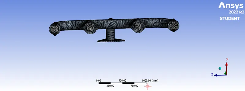
The exhaust post model is updated in the ansys workbench after the completeion of meshing.

SETUP:
In the setup workbench use physics bar tool the energy equation is used.

the meshing is displayed in the fluent is shown below:

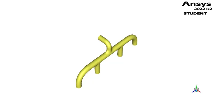
in the energy equation use K-epsilion equation is sselected.
The view of the exhaust post model is changed for our convienet.
Now set the boundary condition of the exhaust posst model.
in result deck - countour - new - velocity - create, the contour lines are generated.
after set the Velocity in the exhaust post model is 5m/s and the temperature of the model is 300kelvin.
the boundary condition of the exhaust post model, in the hybrid method the model is inizalited.
now set the number of iteration is 150. after set the animation of the exhaust post model.
now run and calculate the result.

the resuidal graph of the flow on the exhaust port :

the lines are x-velocity,y-velocity ,z-velocity , energy , k-epsilon.

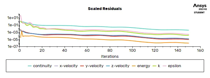
after this process is compelete the scale residual and the contour results are showed.

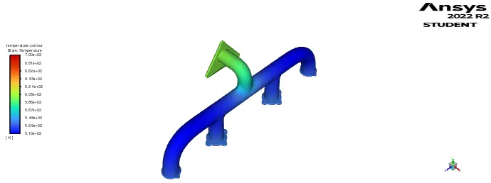
the temperature contour of the flow in the exhust port is shown below:

this contour helps to the analysis of the port where the high temperature results and how the flow with temperature is analysis by this temperture contour:

the velocity contour of the flow in the exhaust port is shown below,which helps to get a deep analysis and about the flow speed and veocity is analysed easily by this contour.

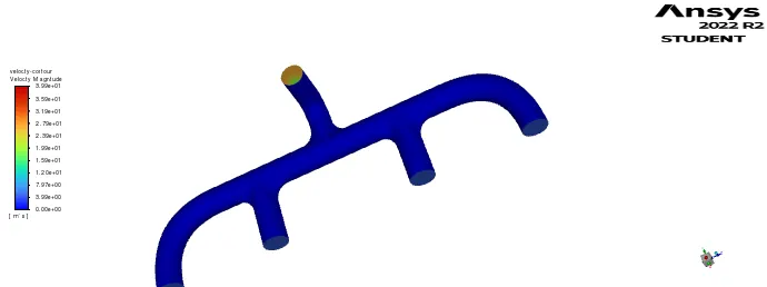
the exhaust post of the model is updated in ansys workbench.

RESULT:

After the model is updated in the ansys workbench the result(cfd post) is opened .

the visuvalization of the flow in the exhaust port is shown in the streamline flow.in oreder to know the direction of the flow and helps to determine the changes happened in the flow.

so the diagram for the streamline in the exhaust port is shown below:

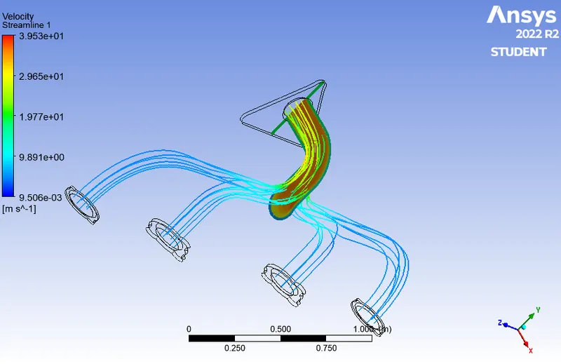
In the compost workbench create the plate in the center of the exhaust workbench.
the transperance of the outer wall convection is done by using rendering option.
In the tool bar by using insert option the plane is created at the exit of the exhaust post so it makes the heat transfer coefficient, velocity, pressure.

the stream line of the exhaust post is generated in order to inspect the fluid flow of the model.

ANSWERS:

1. Give a brief description of why and where a CHT analysis is used.

The Conjugate Heat Transfer (CHT) analysis type allows for the simulation of heat transfer between solid and fluid domains by exchanging thermal energy at the interfaces between them. Typical applications of this analysis type exist as, but are not limited to, the simulation of heat exchangers, cooling of electronic equipment, and general-purpose cooling and heating systems.

The Conjugate Heat Transfer (CHT) analysis is used because ,it gives Efficiently combining heat transfer in fluids and solids is the key to designing effective coolers, heaters, or heat exchangers. The fluid usually plays the role of energy carrier on large distances. Forced convection is the most common way to achieve high heat transfer rate.

Conjugate Heat Transfer(CHT) Applications:

Effective Heat Transfer

Efficiently combining heat transfer in fluids and solids is the key to designing effective coolers, heaters, or heat exchangers.

The fluid usually plays the role of energy carrier on large distances. Forced convection is the most common way to achieve high heat transfer rate. In some applications, the performances are further improved by combining convection with phase change (for example liquid water to vapor phase change).

Even so, solids are also needed, in particular to separate fluids in a heat exchanger so that fluids exchange energy without being mixed.

Energy Savings

Heat transfer in fluids and solids can also be combined to minimize heat losses in various devices. Because most gases (especially at low pressure) have small thermal conductivities, they can be used as thermal insulators… provided they are not in motion. In many situations, gas is preferred to other material due to its low weight. In any case, it is important to limit the heat transfer by convection, in particular by reducing the natural convection effects. Judicious positioning of walls and use of small cavities helps to control the natural convection. Applied at the micro scale, the principle leads to the insulation foam concept where tiny cavities of air (bubbles) are trapped in the foam material (e.g. polyurethane), which combines high insulation performances with light weight.

Forced Convection

The forced convection regime corresponds to configurations where the flow is driven by external phenomena (e.g. wind) or devices (e.g. fans, pumps) that dominate buoyancy effects.

Natural Convection

The natural convection regime corresponds to configurations where the flow is driven by buoyancy effects. Depending on the expected thermal performance, the natural convection can be beneficial (e.g. cooling application) or negative (e.g. natural convection in insulation layer.

2.Maintain the y+ value according to the turbulence model and justify the results.

y+ is a non-dimensional distance. It is often used to describe how coarse or fine a mesh is for a particular flow pattern. It is important in turbulence modeling to determine the proper size of the cells near domain walls. The turbulence model wall laws have restrictions on the y+ value at the wall

Generally when you building grid for RANS model of k-epsilon the target value of y⁺ should be between 30 and 300 .

3.Calculate the wall/surface heat transfer coefficient on the internal solid surface & show the velocity & temperature contours in appropriate areas.

The velocity and temperature contour is created for this flow in the exhaust port and displayed in the fluent section.by the help of the velocty and temperature contour the breif analysis about the flow is determined and calculated.

the flow velocity and the wall heat transfer co efficient on the internal solid surface is analysied by the help of the CFD post in the result section of the ansys workench.

the velocity is visualized in the outlet by iserting a plate in the outlet region, that diagram is shown below:

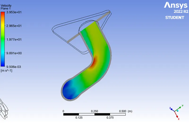
the velocity changes are visible in the plate and that is easy to analysis.

the temperature of the flow in the exhaust port is also seen in the outlet plate , by this the analysis of the temperature difference between the inlet and outlet is determined.

the temperature is shown in the outlet plate below:

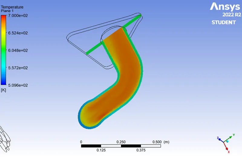
this is the velocity and temperature contours and distribution inside the solid .

4.How would you verify if the HTC predictions from the simulations are right? On what factors does the accuracy of the prediction depend on?

• The Nusselt number is the ratio of convective to conductive heat transfer across a boundary.

• We need to make sure that share topology is set to share.Only then the meshing is going to be uniform and with perfect connectivity.
• We need to select exact turbulent model.As it is wall bounded flow k- omega SST will be very much suitable.And when selecting the turbulence model selecting exact Y+ value also important.
• Since at the interface it is very important as we want to calculate the heat transfer at that place we need to take that region and create inflation layers so that flow is captured exactly and the values are calculated exactly.
• We need to enable sharein the work bench and click share .This is very important if you dont do this step you will not see the single interface between them.So this particular step takes care of creating the interfaces ,so that you will have one interface between your solid volume or block and fluid block.

By this process the simulation of the exhaust port is completed succesfully.