Week 4 - CHT Analysis on Exhaust port

AIM- Steady state CHT analysis on exhaust port with detailed Theory,Maintained Y+ model , Contours and conclusion of results.

THEORY

1. Conjugate heat transfer(CHT)

Conjugate heat transfer analysis is based on a mathematically structured problem, Which describes the heat transfer between body and fluid internaly or extrenaly as result of interaction between two Body mediums. At matching interface the details are provided for temperature distribution and heat flux along the interface eliminating the need of calculating the heat transfer coefficient.Which can be calculated later.

One of simplest way yo realize the conjugation is through numerical methods. the boundary conditions for the fluid and solid interface is set and solved through iterations method. There are nno right guesses for the values of initial boundary condition for the convergence except through the hit and trial method.

CHT approach has an advantages over FE thermal analysis in that wall heat transfer coefficients and theire local variations on surfaces which are directly calcuated within the model rather than based on simplfied empirical calculations. the CHT approach ,therefore has benifits for those applications where heat transfer is either non-uniform or difficult to calcualte.

CHT has become a powerfull tool in recent times as it provides answer to different natural phenomenon engineering systems in different areas like Aerospace, Nuclear reactors, thermal goods,medicinal to many other fields.

Applications

EFECTIVE HEAT TRANSFERS
Efficiently combining heat transfer in fluids and solids is key to design effective coolers,heatersetc. The fluid is energy carrier on larger distances. Forced convection is the most common way to achieve a high heat transfer rate. The performances are further improved by combining convection with phase change.

ENERGY SAVINGS
Heat transfer in fluids and solids can also be combined to minimize heat losses in various devices. Most electronical equipments are source of generating heat to minimize this loss we use these mediums to prevent energy loss in form of heat. Mostly we uses gases as they have low thermal conductivity and can be used as insulators or mediums like water and air to cool down the process to optimum temperature as energy generations is maximum when the process happens in optimum suitable temperature according to material.

SOLVING AND MODELING APPROACH

• The exhaust port is imported into Spaceclaim in ANSYS FLUENT
• The exhaust port is a three-dimensional model containing four inlets and one outlet despite having isothermal boundary conditions and a uniform flow rate at four inlets, The model cannot be cut into two half to save computaional time beacuse of its assymmetrical bosy type. So, whole body is meshed.
• CHT requires both the solid and liquid volume under consideration,we open volume extract in spaceclaim by selcting inner edges.
• Both solid and fluid body is moved into 1 component.
• Share topology is created .So, all data can be moved smoothely from fluid to solid body without any hinderence or delay.
• The Exhaust port is then opened in Mesh and genrate mesh for 150mm then refined mesh for 17 mm.
• The name selctions is done Inlets, Outlets,Convection layer & inflation layer.
• We use inflation for inflation layer using Y+ model which is calculated to be 0.59mm(shown below)
• After updating mesh we open geometry to solve, Where we use steady and pressure based model and viscous model of k-Omega(As Omega is more suitable for conditons near wall)
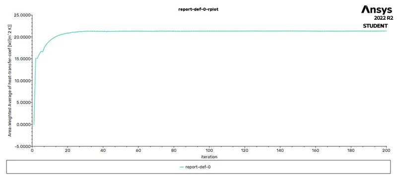
• We genrate plot for surface heat transfer coefficient by using defination.
• We initialise and then run solution for 300 iterations.

PRE-PROCESSING AND SOLVER SETTING

CASE-I( MESH SIZE= 150MM)

Geometry

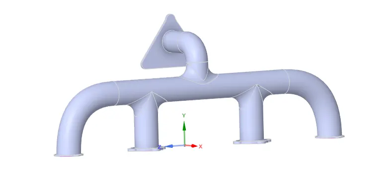
Fluid volume extraction

Extracting solid and fluid volume and moving into 1 component named (Exhaution port) As shown below

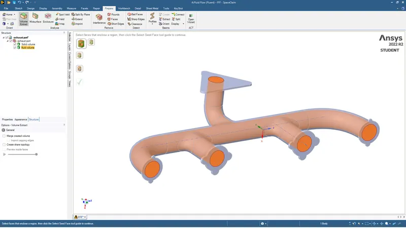
Share topology

It is done so data can be shared form fluid to solid vice-versa . Without this step we wouldn't be able to see surface heat transfer coefficient.

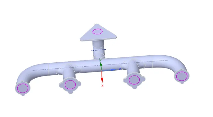
After completing sharing it will show purple as above where boundary is shared.

Meshing

Here we import finished geometry into meshing abd generate mesh for default 150 mm.

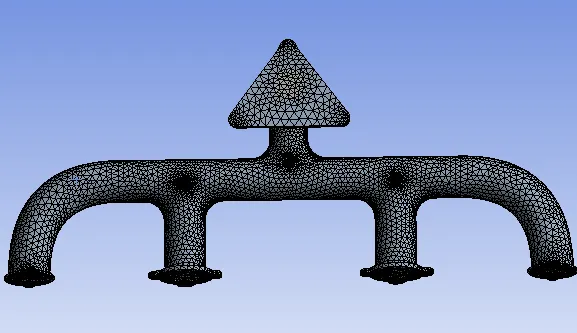
Named selection

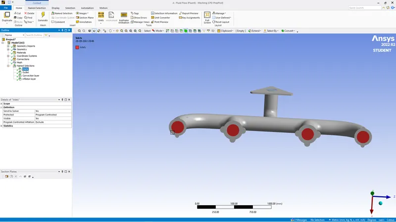
Inlet= velocity @5m/s

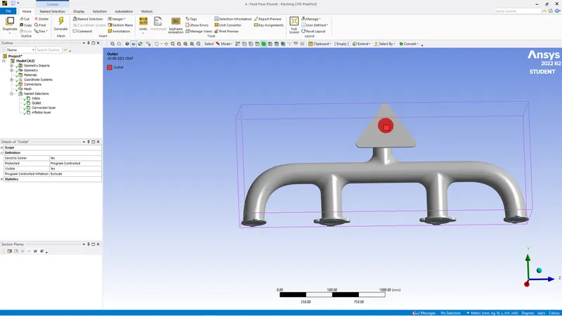
Outlet

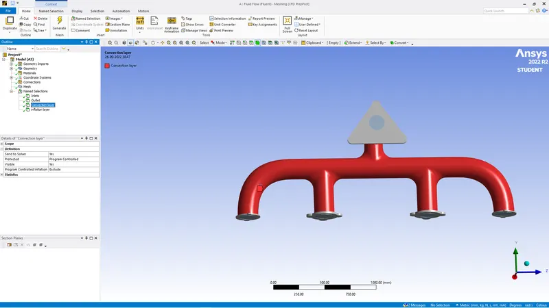
Outer wall convection( Heat transfer coeffiecient 20 `W/(m^2K)` free stream temperature 300k)

Inflation layer

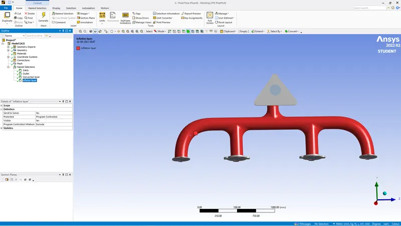
Adding inflation layer according to Y+ model

We calcualte Y+ model using Y+ calculator

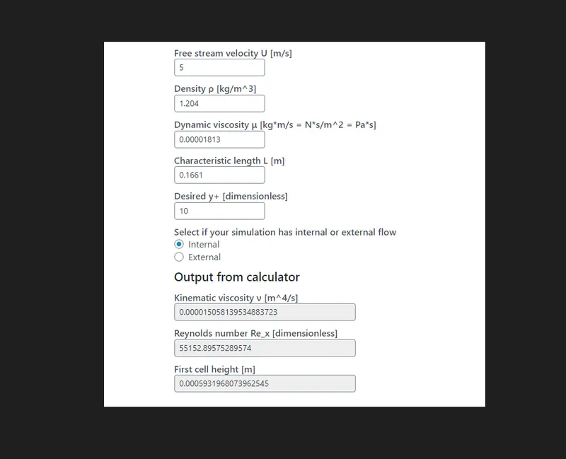
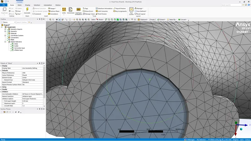
We give Y+ data in inflation where we choose the name slection process and choose inflation layer.

Setup for solver

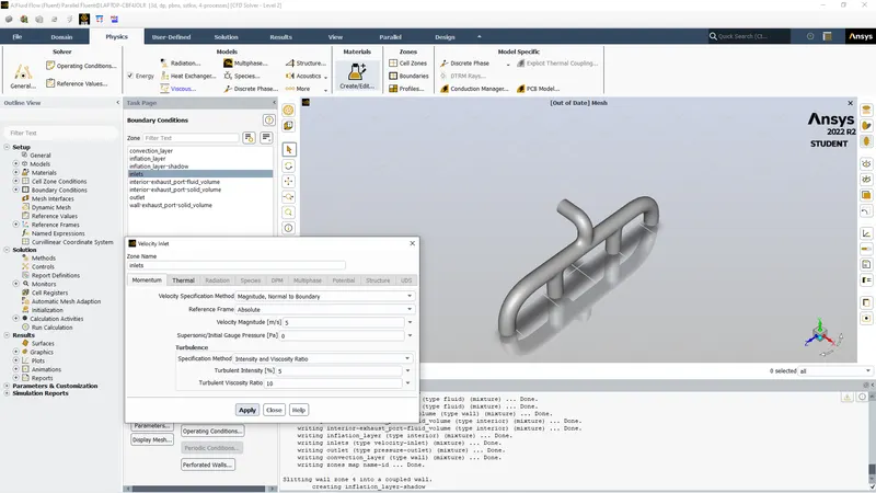
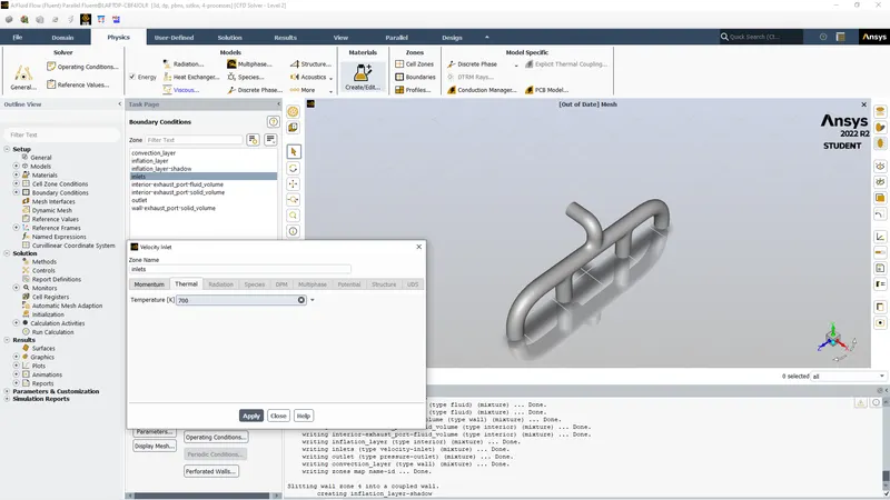
Inlet boundary condition

Type= Velocity inlet
Velocity = 5m/s
Temperature= 700K

Outlet boundary condition

Type= Pressure outlet
Gauge pressure= 0 Pa

Outer wall convertion( convection layer)

Type= Wall
Thermal condition= convection
Heat transfer coefficient: 20`W/(m^2K)`

Rest boundary condition remain as default.

Energy equations: It is turned on as we need temperature data.

Viscous model: k-omega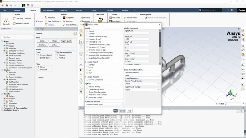

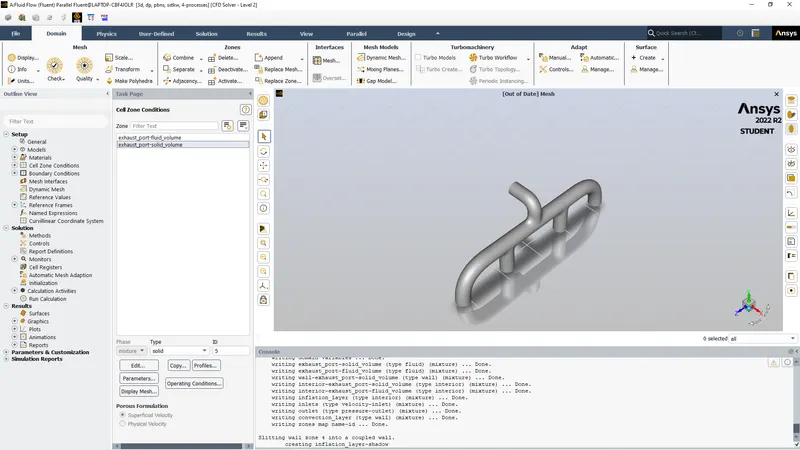
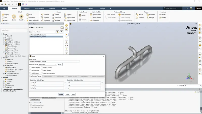
We need to change the solid type body in cell zone

Result for Case-I

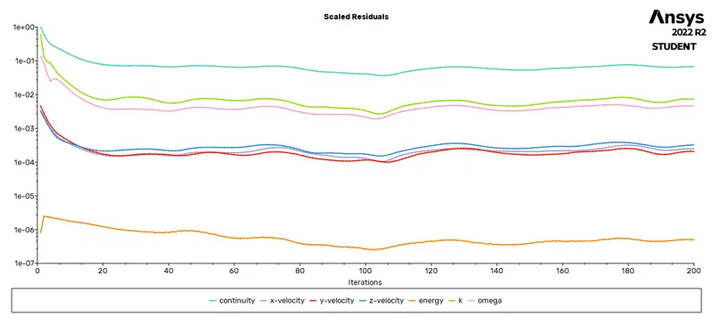
Residual plot

Surface heat transfer coefficient

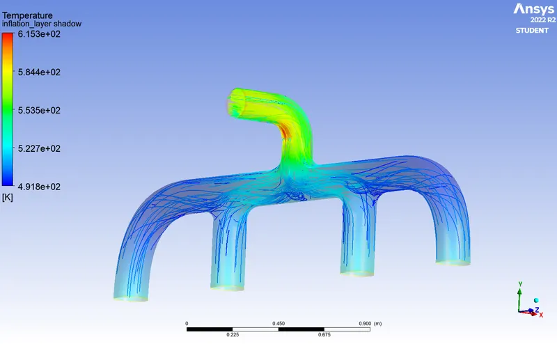
Temperature contour, volume rendering,Body

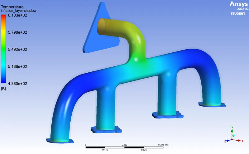
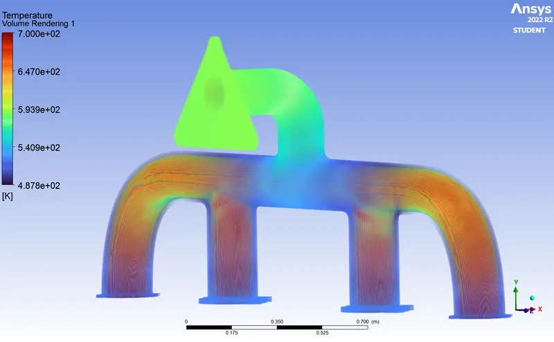
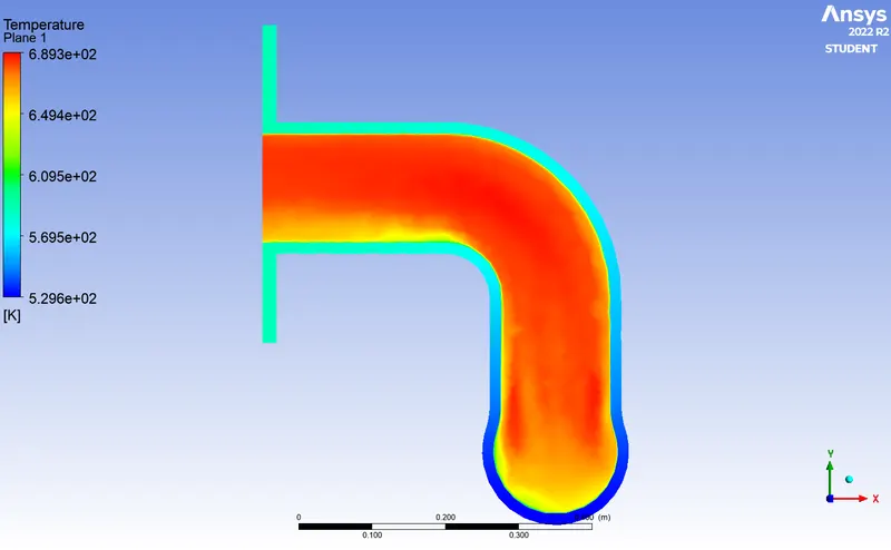
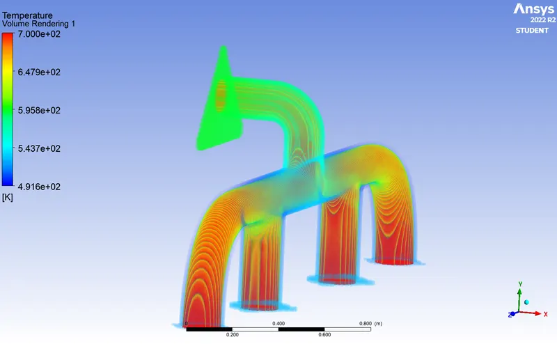
The colour near wall represents the heat transfer due to convection and pipe temperature is affected by fluid temperature in pipe.

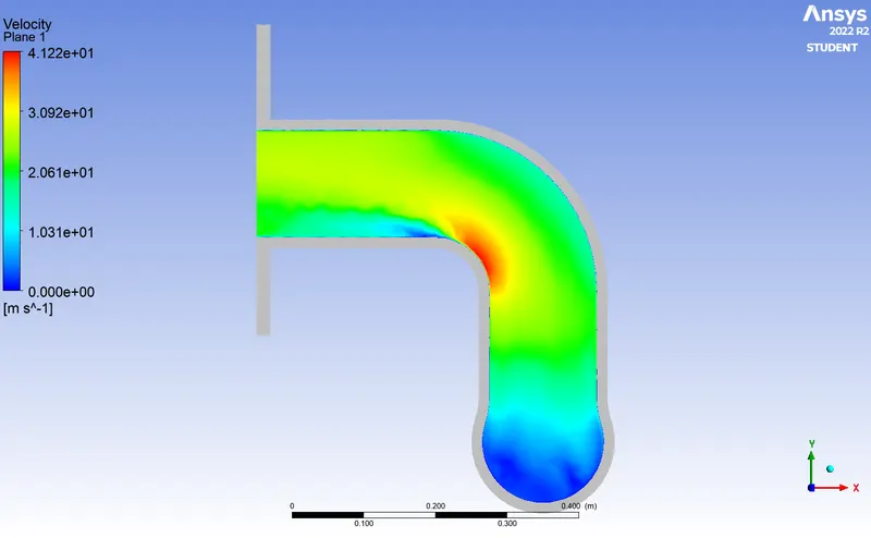
Velocity contour, streamlines

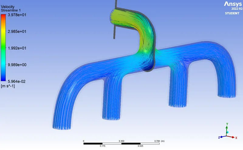
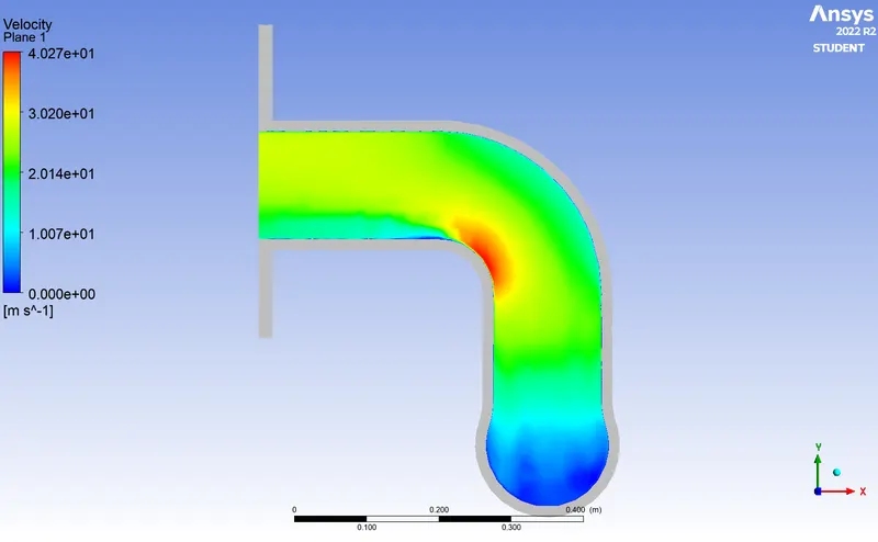
As we can see the velocity low near wall due to friction is most near walls and in stream lines show increase in velocity as 4 inlets velocity is increases due to more discharge as there is only 1 outlet.

CASE-II( Mesh = 17mm)

Meshing length is changed to 17mm and mesh is generated

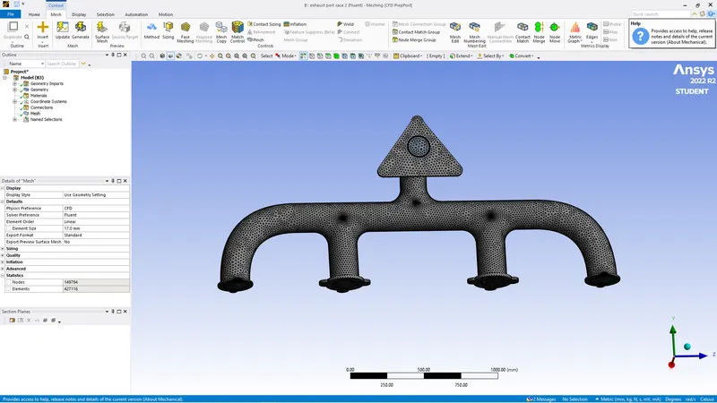
We then open solver to solve for same process .

Results Case-II

Residual plot

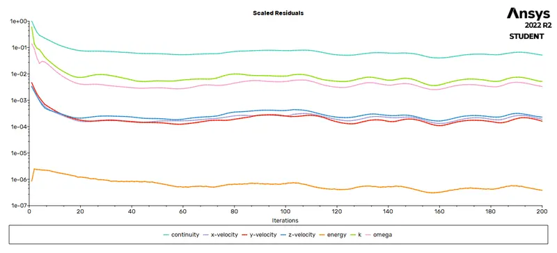
Surface heat transfer coefficient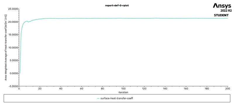

Temperature contour,Volume rendering,Body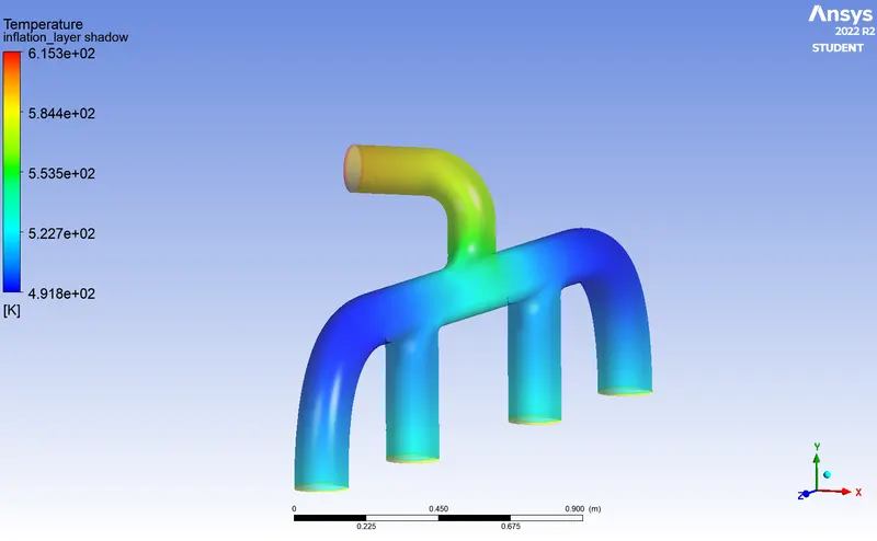

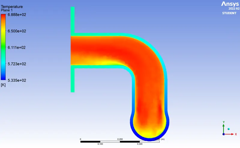
Velocity contour ,Streamlines

Surface heat transfer

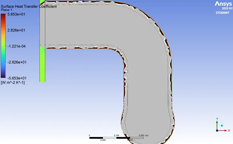
The Wall surface shows Heat transfer coefficientand changes caused due to hot fluid.

COMPARISSION OF RESULTS AND ITS SIGNIFICANCS

GRID INDEPENDENT STUDY	MESH SIZE	NO. OF ELEMENTS	HEAT TRANSFER COEFFICEINT(h)
CASE 1	150MM	2,42,630	21.35
CASE 2	17MM	4,70,689	21.34

In both cases few properties remain constant

Conductivity(k)= 0.0242
Cp= 1006.43
Density= 1.225
diameter= 0.166
Reynolds number = 55119.8

The results got improved with mesh size improvement just that in this case the outcome was not so drastiaclly dependent on grid sizing so results didint vary at much but if we decrese more mesh size it will vary more but we cant conduct that due to student version only allow 5lakh elements.

Analytical Heat transfer coefficient

We use formula

Conductivity(k)= 0.0242
Cp= 1006.43
Density= 1.225
Diameter(D)= 0.166
Reynolds number(Re) = 55119.8
Prandtl number(Pr)= 0.79

Nu(nusselt number)= `(h*D)/K`

Nu= `0.023*Re^0.8*Pr^0.3`

h= 20.1

The analytical data for heat transfer coefficient is 20.1 & data of solver is 21.34 so the result is almost accurate.

Conclusions

• The CHT analysis on exhaust port was simulated succesfully on ANSYS _FLUENT.
• The Result is almost accurate as comparable to analytical data as shown above.
• If we improve the Grid quality and size . We can acchieve even better result .
• Even after changing mesh size from 150 mm to 17 mm the result didn't differ much that show we need even more smaller size to find better solution.
• K- omega solver give appropriate result as it is more suited to Wall based solution rather than k-epsillon which suited to outlet flow.

Factors influenced Accuracy

• Mesh quality greatlt impacts the accuracy of predicted value from our simulations which can be observed from above contous and maximum values of related parameteres like velocity and haeta transfer coefficent
• Appropriate Y+ value helps in caalculating total layer thickness form wall of the better capturing of effects of near walls. In this case HTC.
• Inflation layers and boundary conditions.
• appropriate solvers like in this case k-omega as explained in conclusion.