Week 4 - CHT Analysis on Exhaust port

challenge 4

Aim: - cfd simulation of exhaust port and calculation of convection heat transfer coefficient for outer surface

Objective: -

1. Give a brief description of why and where a CHT analysis is used.
2. Maintain the y+ value according to the turbulence model and justify the results.
3. Calculate the wall/surface heat transfer coefficient on the internal solid surface & show the velocity & temperature contours in appropriate areas.
4. How would you verify if the HTC predictions from the simulations are right? On what factors does the accuracy of the prediction depend on?

Introduction: - The Conjugate Heat Transfer (CHT) analysis type allows for the simulation of heat transfer between solid and fluid domains by exchanging thermal energy at the interfaces between them. Typical applications of this analysis type exist as, but are not limited to, the simulation of heat exchangers, cooling of electronic equipment, and general-purpose cooling and heating systems.

To have analytical or numerical prediction of heat transfer coefficient close to experimentally obtained values, one must focus on conjugating the boundary condition at the fluid–solid interface through coupled heat transfer analysis. Such a coupled field study is termed as Conjugate Heat Transfer (CHT) analysis

CHT studies involving fluid and solid domains. Coupled field analysis or specifically CHT analysis is essential in a situation where solution domain consists of more than one sub-domains in which heat transfer is governed by different differential equations. In such a case suitable governing equations are to be solved in the respective sub-domains and these solutions need to be conjugated at the interfaces of sub-domains. Aforesaid explicit solution seeking and coupling are also inevitable even if the heat transfer is governed by same set of differential equations, but sub-domains are having dissimilar material properties.

Application: - Applications of CHT analysis is unaccountable. Most promising application of CHT study is found to be convective cooling of mechanical, electrical and electronic components. Substantial number of CHT studies in the field of turbine blade cooling, electronic circuit cooling and alternator winding cooling are available. CHT technique also got application in sensor design, heat exchanger analysis, space vehicle design and even analysis of biosystems. The coupling of CHT codes with structural solvers extends the application envelope of CHT technique. Study of ablation cooling of re-entry vehicle is an important area where CHT technique can be applied efficiently. Researchers around the globe are working towards the improvement of CHT coupling technique and extension of its application field.

Solving & Modelling approach: -

Geometry setup: -

• File is imported to space claim application the repair if any are there using repair section command
• To Extract fluid volume extract volume command is used
• Extracted fluid volume and already present solid volumes are transferred to same components and empty components were deleted
• To share information from one volume to another volume share topology has to be enabled and from workbench section share command is used and topology is shared and close the splaceclaim application

Mesh

• name inlet, outlet, outer wall and inflation layer
• Initially direct mesh is generated to run he basic simulation
• In refined mesh inflation layer is added to inflation layer named component and body sizing is done for outer wall and element size is decreased to 50 mm
• And the mesh application is closed

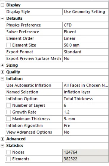
fig 1 details for refined mesh

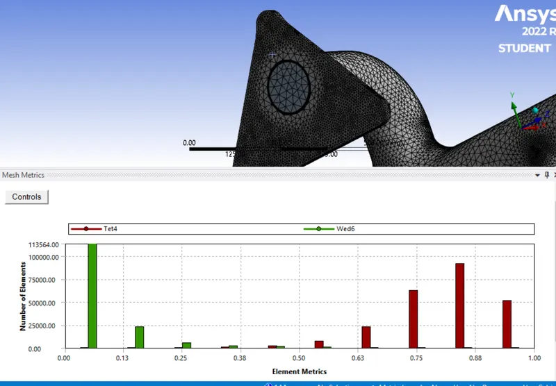
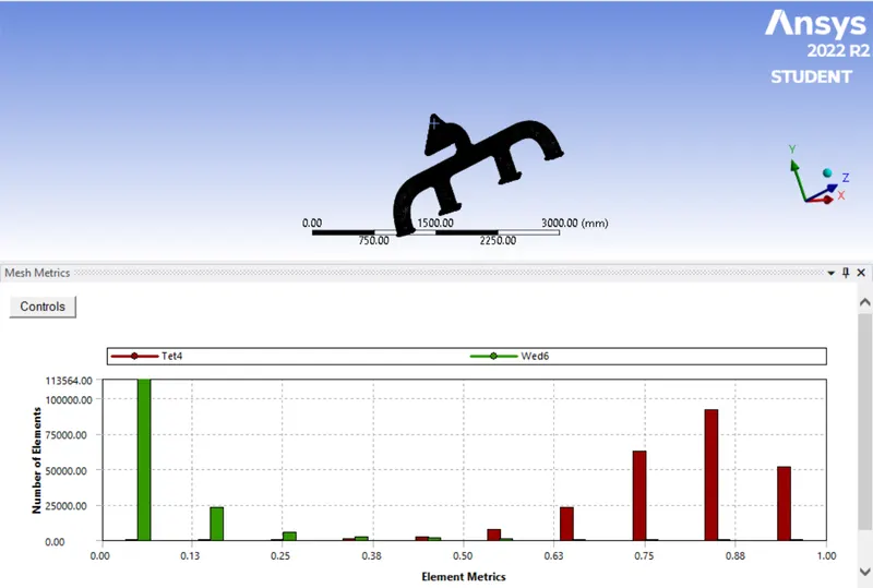
fig 2 mesh qaulity for refined mesh

Setup

Check for mesh

In setup section select energy and viscous model as k epsilon model

In martials for fluid select air and for solid aluminium

Boundary conditions inlet with 5m/s velocity and temp as 700 k

Outer wall convection and heat coefficient as 20w/m^2 k

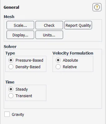
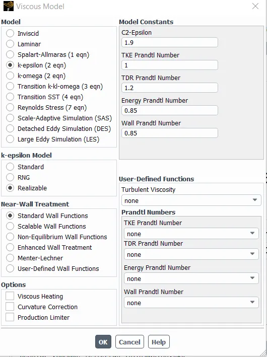
fig 3 setup parameters for solution

Solution hybrid and initialize the solution and in post process create a contour for temp at outer wall of the exhaust port and create animation for contour

And calculates for 200 iterations

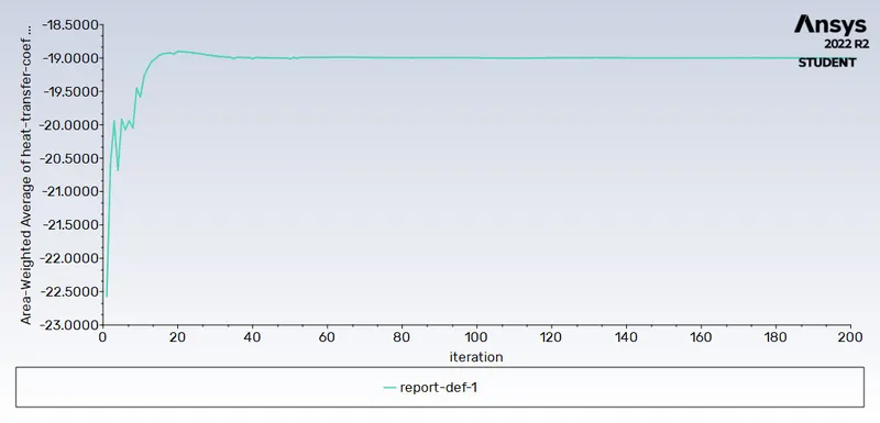
fig 4 wall heat coeffeint for outer wall

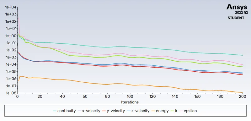
fig 5 residuel moniter

post processing

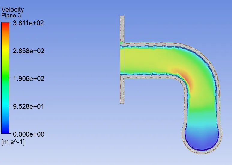
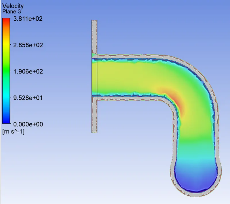
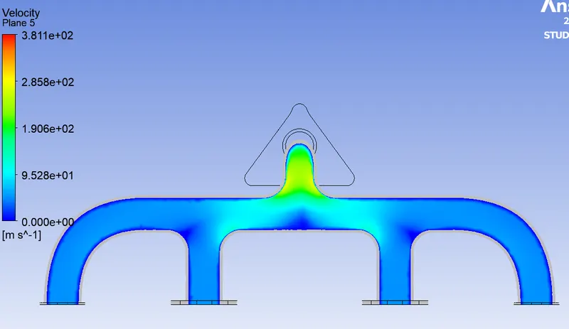
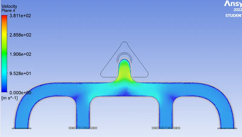
fig 6 velocity andsuface heat coeffent results

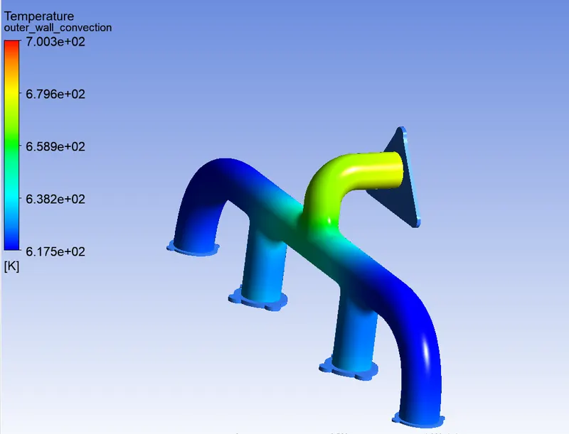
fig 7 temp result contour

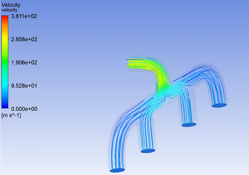
fig 8 velocity stream line

refines mesh result with k epsilon model

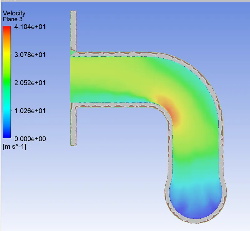
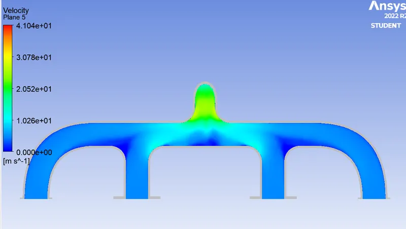
fig 9 refined mesh velocity and surface heat coeffeint result

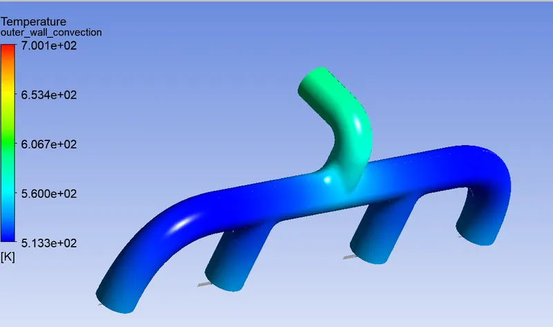
fig 10 refined mesh temp result contour

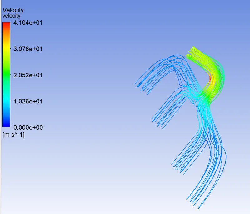
fig 11 refined mesh velocity stream line

k eplsilon model result

fig 12 heat transfer coeefient and residuel montor

heat transfer coeefient 19.01

K OMEGA with simple method solution

Y+ calculation

reynolds number calculation

`Re= (rho *v*D)/mu`

Re =(1.225*5*0.15)/(1.78*10^-5)

Re=51335.5

friction coeffient

`C_f=0.026/(Re)^(1/7`

c_f=0.0055

`tau_w=(c_f*rho*v^2)/2`

=0.084

frition velocity

`u^*=sqrt(tau_2/rho)`

=0.26 m/s

`Y^+=(delta y*u^**rho)/mu`

=89.66

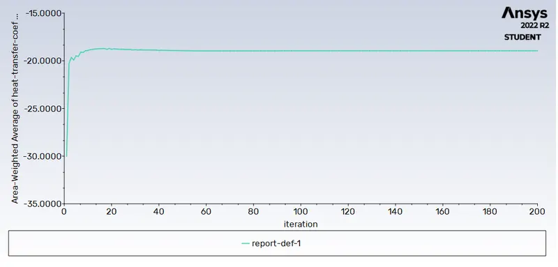
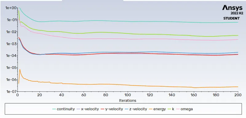
fig 13 heat transfer coeefient and residuel montor simple method

heat ransfer coeefient 18.97

simplec

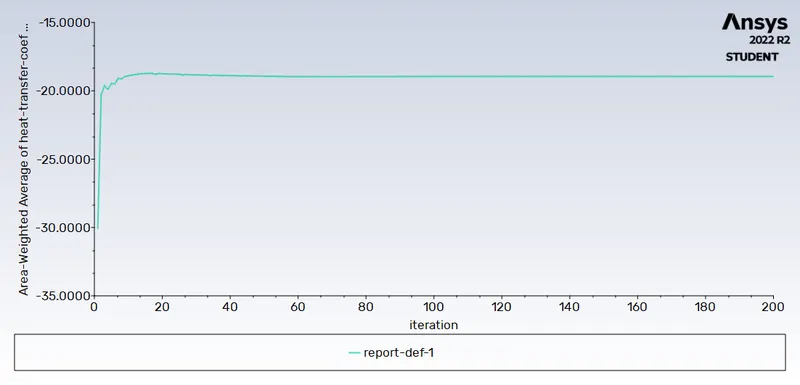
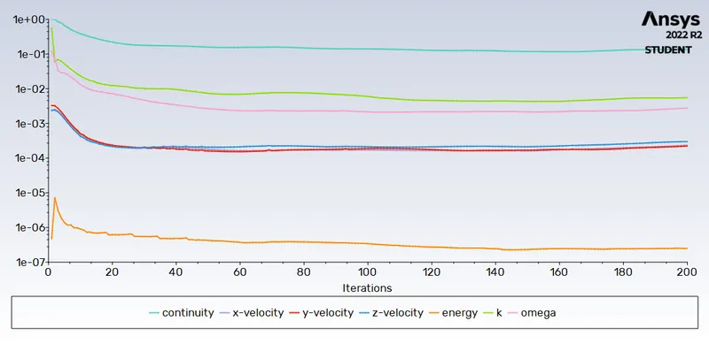
fig 14 heat transfer coeefient and residuel montor simplec method

heat ransfer coeefient 19.03

piso

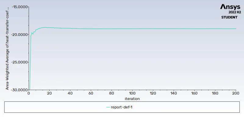
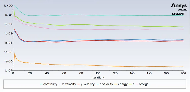
fig 13 heat transfer coeefient and residuel montor PISO method

heat ransfer coeefient 18.81

coupled

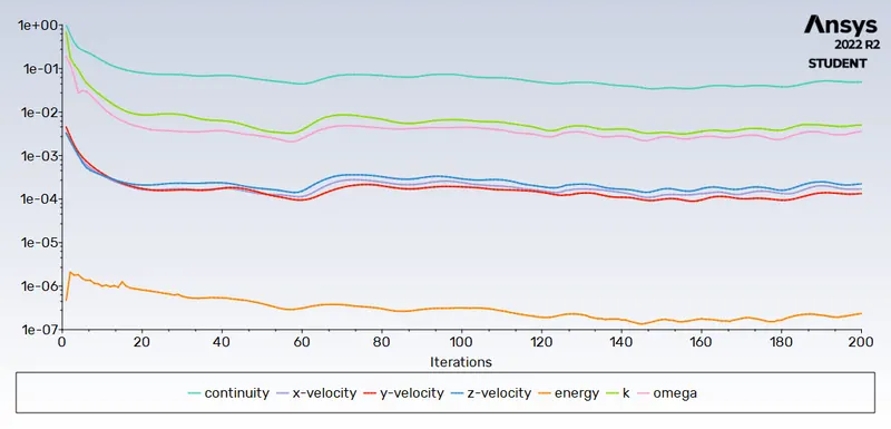
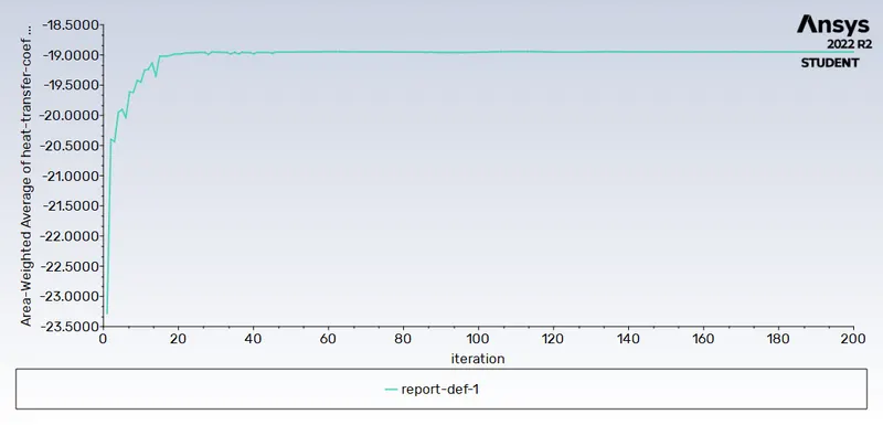
fig 13 heat transfer coeefient and residuel montor coupled method

heat ransfer coeefient 18.95

Method	Model	k in W/(m^2 k)
coupled	K epsilon	19.01
simple	K omega	18.97
Simplec	K omega	19.03
PISO	K omega	18.81
Coupled	K omega	18.95

numerical calculation of heat transfer coeffencent

Prandtl number

`Pr=mu*C_p/k`

=1.789*10^(-5)*1006.43/0.0242

=0.744

`Nu=0.0265*Re^(0.8 )*Pr^(0.3)`

`Nu=0.0265*511355.5^(0.8)*0.744^(0.3)`

Nu=142.25

`h=Nu*k/D`

h=142.25*0.0242/0.15

h=22.01 W/(m^2*k)

conclusion

from temprature contour it ca be seen that temp at inlet side is less compared to outlet side were as the temp at in let is more than the outlet temp this is happening because there is not enough time to convect tthe heat from fluids to the outer wall as the fluid moved in side the volume it gets enough time and heat transfer takes place

at inlet the the raynld no is less as the fluid move inside the velocity starts to increasee at juction of all port fluid hence ther can be seen higher heat transfer and velocity is also high at that point

from above to figuers it can be seen that the velocity at corner is more then the all over the body so is the heat transfer coeffient

but in first figre without inflation layer the heatransfer coeefent looks bet odd but with inflation layer the heattrasfer coeefent looks good

from numerical method the heat transfer coeefent is 22.01 W/(m^2*k)

but with cfd analysis the heat transfer coeffient is around 19 W/(m^2*k)

reference

https://s3.amazonaws.com/suncam/docs/119.pdf

https://www.cadence.com/en_US/home/tools/system-analysis/computational-fluid-dynamics/y-plus.html