Week 4 - CHT Analysis on Exhaust port
Objectives:
Give a brief description of why and where a CHT analysis is used.
Maintain the y+ value according to the turbulence model and justify the results.
Calculate the wall/surface heat transfer coefficient on the internal solid surface & show the velocity & temperature contours in appropriate areas.
How would you verify if the HTC predictions from the simulations are right? On what factors does the accuracy of the prediction depend on?
SOLUTION
AIM:
To perform the simulation of Conjugate heat transfer analysis on given exhaust port geometry by using ANSYS FLUENT.
OBJECTIVE:
- To study the importance of Conjugate heat transfer analysis and importance of y+ value during meshing of the components.
- To perform the simulation of Conjugate heat transfer analysis on given exhaust port geometry by using ANSYS FLUENT.
- To calculate the wall heat transfer coefficient and to plot velocity and temperature contours of baseline and fine mesh simulations.
THEORY:
Conjugate Heat Transfer Analysis -
Conjugate heat transfer analysis (CHT) describes the heat transfer due to the interaction of a solid body and fluid flowing over or inside it. Conjugate heat transfer plays a vital role in the modern world ranging from automotive industry, aerospace, cryogenic applications, food processing, cooling of electronic devices, Heat exchanger design etc. CHT analysis provide the temperature distribution, heat transfer contours, heat transfer coefficient, heat flux values at the interface thus one can easily conclude the behaviour of a system.
PROCEDURE:
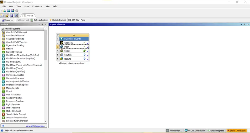
- Open ANSYS Workbench 2022R2 select Fluid Flow (Fluent) from Toolbox.
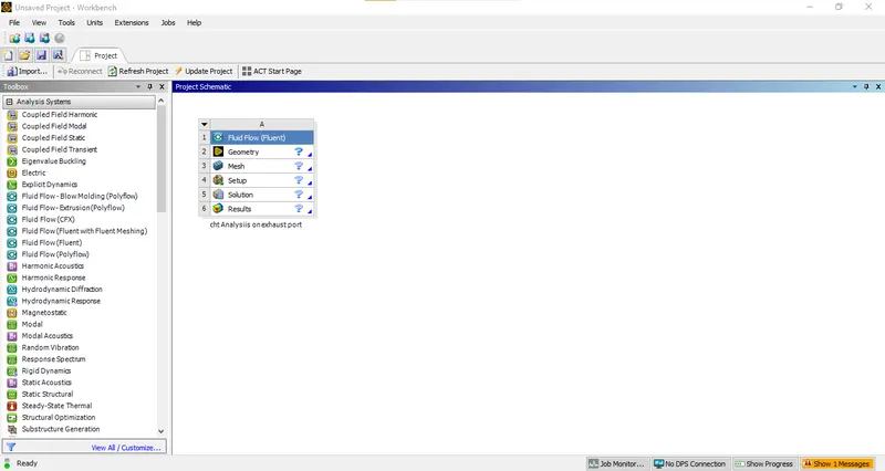
- Rename the file and left click Geometry and select New Spaceclaim Geometry.
- Open the geometry STEP or SLDPRT of the geometry in spaceclaim.
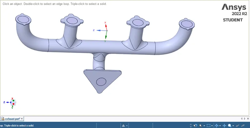
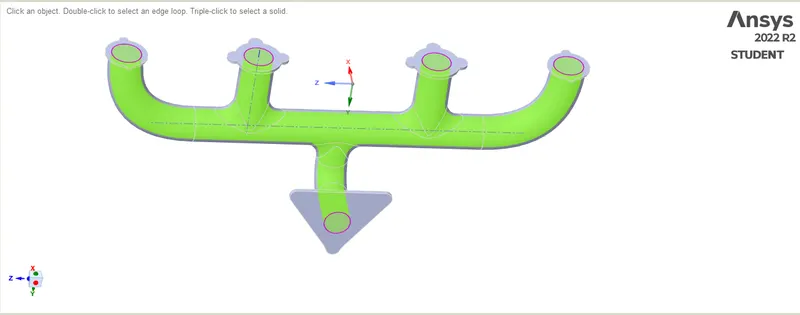
- Extract the fluid volume by selecting Extract Volume option from Prepare menu on top bar. Then select the edges and click the tick mark now a new volume is created and which can be visible on tree. Name this volume as fluid volume and geometry as solid volume. Also delete the duplicate edges or entities present in the geometry by selecting Extra Edges option from Repair menu.
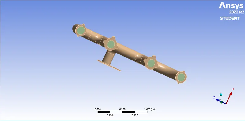
- From the Analysis section share topology should be turned on as Share and perform the same by selecting share option from Workbench menu
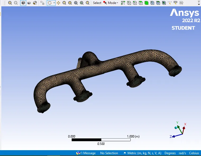
- Close SpaceClaim and double click on Mesh. Meshing window will appear. Mark Inlet, Outlet, Outer wall convection on geometry by right clicking each part and selecting Create Name Selection. Now select the mesh from the tree and generate mesh with an appropriate element size (0.15m) to get a base-line meshing on the surface of geometry. The figure shown below show the geometry after meshing.
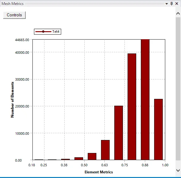
Element Quality
Close Meshing and double click on Setup, select Double Precision and Fluent window will open. Check all the values and make necessary correction if needed.
SETUP
Select appropriate conditions mentioned below.
Solver - Pressure Based
Viscous - k-epsilon model
Energy - On
Material - Fluid, Air - Solid , Aluminum
Cell Zone Conditions
Volume - Fluid - Air , Solid - Aluminum
Boundary Conditions
Inlet - Velocity Inlet, Velocity = 5m/s, Temperature = 700K
Outer wall convection- Wall
Outlet - Pressure Outlet
Define Area weighted average of heat transfer coefficient and Outlet temperature.
Solution Initialization - Hybrid Initialization.
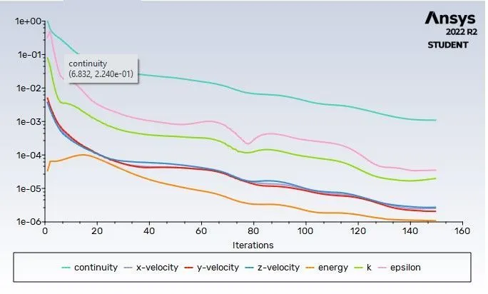
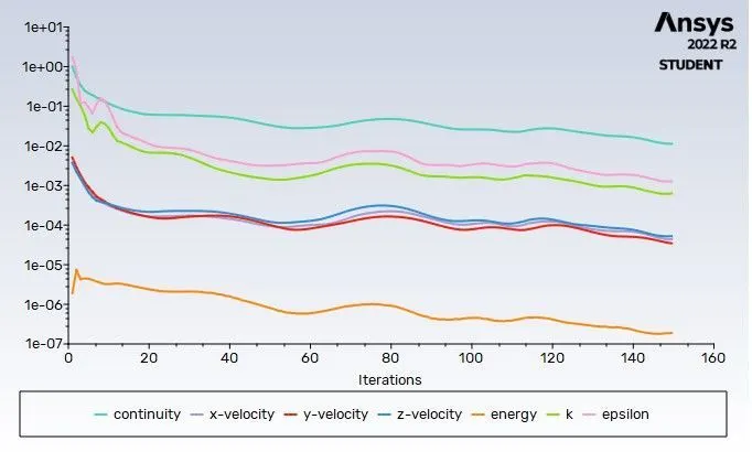
After assigning all the factors click on Run Calculation and set number of iteration and calculate.The figure below shows the residual plot after calculation.
First Layer Thickness Calculation.
In the question it is mentioned to consider the flow is turbulent. So k-epsilon turbulence model is considered for the simulation. y+ value for the k-epsilon model is in between 30-300. As wall heat transfer coefficient is needed to evaluate y+ value is considered as 30. By using y+ value calculator first layer thickness is evaluated.
y+ value - 30
Density of air - 1.225 kg/m3
Viscosity - 1.7894e-5 kg/ms
Length - 0.17 m (Inner diameter)
Velocity - 5 m/s
Upon calcuation first layer thickness obtained is 1.5mm
Residual plot obtained for fine meshing case is shown below.
The results obtained are discussed in the next session.
RESULTS
CASE-1 - BASE LINE MESHING
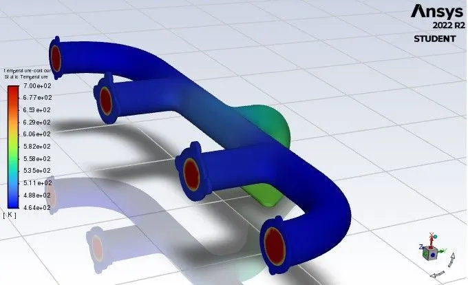
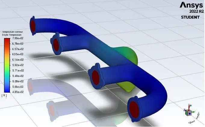
Temperature Contour
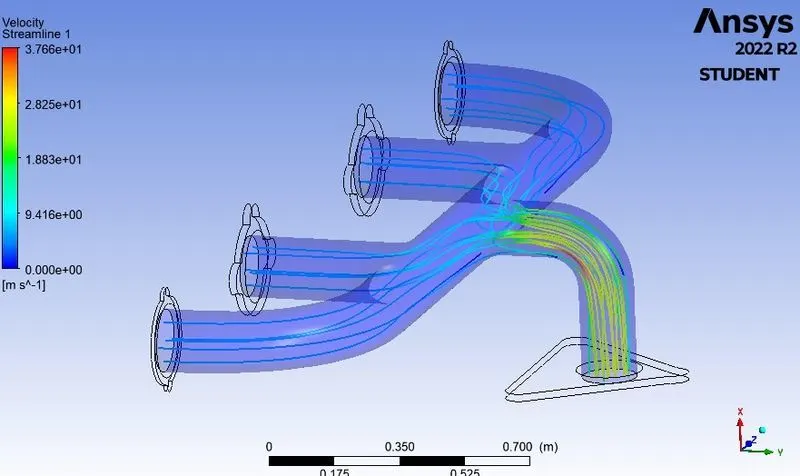
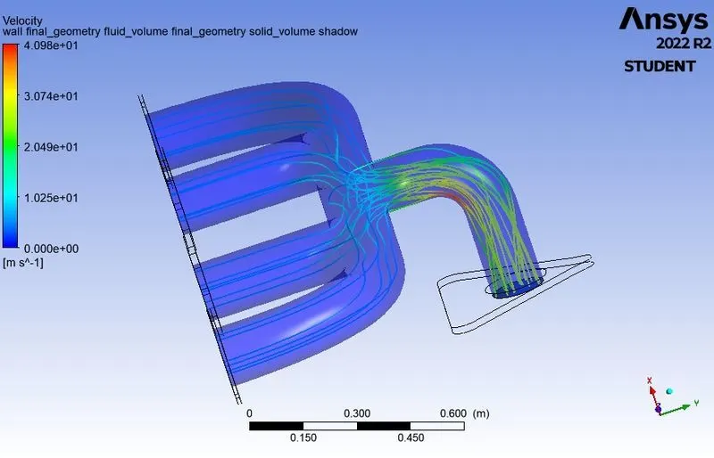
Velocity Contour
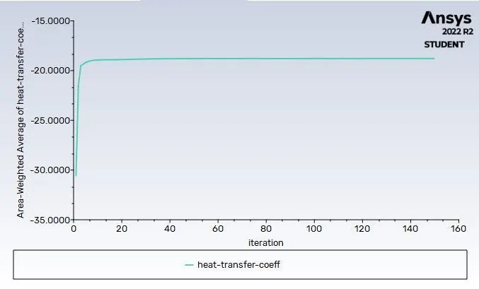
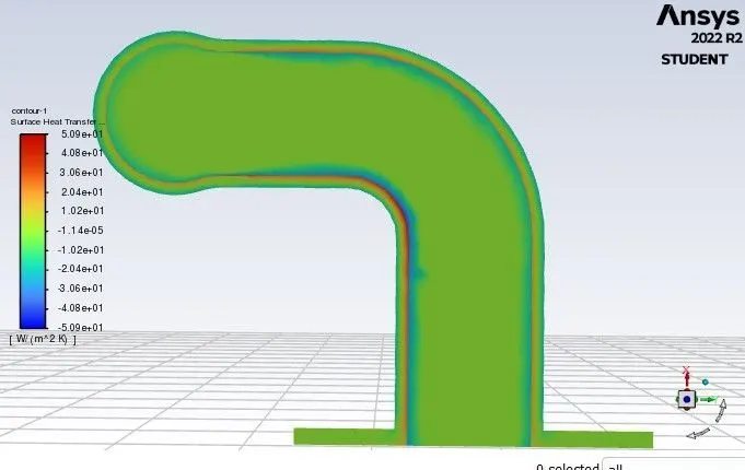
Heat transfer coefficient
Surface heat transfer coefficient contour
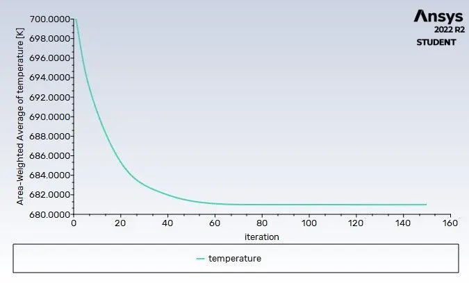
Outlet Temperature
CASE-2 - FINE MESHING
Temperature Contour
Velocity Contour
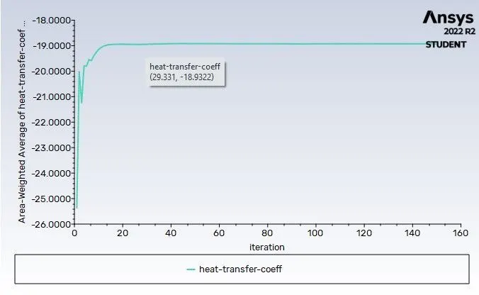
Heat transfer coefficient
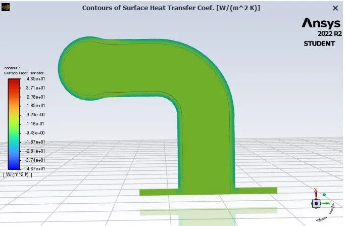
Surface heat transfer coefficient contour
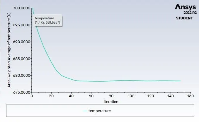
Outlet Temperature
| Cell Count | Outlet Temperature | Heat transfer coefficient | |
| Part - 1 (Baseline Meshing) |
137836 |
680.98 K | 18.79 W/m2.K |
| Part - 2 (Fine Meshing) |
234183 |
678.36 K | 18.92 W/m2.K |
From the above table and figures it is evident that the contours and results obtained are more clear and accurate for fine meshing as compared with baseline meshing. Even though fine meshing take more computational time but the results obtained are accurate. Which can be justified with help of results and contour obtained.
CONCLUSION:
The simulation of of Conjugate heat transfer analysis on given exhaust port geometry was carried out using Ansys Fluent. From the study it is concluded that the results obtained from part 1 are poor as compared to part 2 as in part 2 fine and high quality meshes with inflation layers at the solid - fluid interface are used where as course meshes are used in Part -1. Thus the refined mesh allows produce a clear picture of simulation.