Week 4 - CHT Analysis on Exhaust port

AIM:

To develop a numerical setup for conjugate heat transfer analysis on the exhaust port.

OBJECTIVE:

• Give a brief description of why and where a CHT analysis is used
• Maintain the y+ value according to the turbulence model and justify the results.
• Calculate the wall/surface heat transfer coefficient on the internal solid surface and show the velocity and temperature contours in appropriate areas
• How would you verify if the HTC predictions from the simulations are right? On what factors does the accuracy of the prediction depend on?

INTRODUCTION:

CONJUGATE HEAT TRANSFER:

The Conjugate Heat Transfer (CHT) analysis type allows for the simulation of heat transfer between solid and fluid domains by exchanging thermal energy at the interfaces between them. Typical applications of this analysis type exist as, but are not limited to, the simulation of heat exchangers, cooling of electronic equipment, and general-purpose cooling and heating systems. For example, heat sinks are optimized to combine heat transfer by conduction in the heat sink with the convection in the surrounding fluid.

Heat Transfer by Solids and Fluids

Heat Transfer in a Solid

In most cases, heat transfer in solids, if only due to conduction, is described by Fourier’s law defining the conductive heat flux, q, proportional to the temperature gradient:

`q = − k △ T`

For a time-dependent problem, the temperature field in an immobile solid verifies the following form of the heat equation:

`ρc_p((∂T)/(∂t))=△.(k△T)+q`

Heat Transfer in a Fluid

Due to the fluid motion, three contributions to the heat equation are included:

1. The transport of fluid implies energy transport too, which appears in the heat equation as the convective contribution. Depending on the thermal properties of the fluid and on the flow regime, either the convective or the conductive heat transfer can dominate.
2. The viscous effects of the fluid flow produce fluid heating. This term is often neglected, nevertheless, its contribution is noticeable to fast flow in viscous fluids.
3. As soon as a fluid density is temperature-dependent, a pressure work term contributes to the heat equation. This accounts for the well-known effect that, for example, compressing air produces heat.

APPLICATIONS OF CHT:

Heat exchangers, HVAC, Air-cooled and liquid-cooled engines, Turbochargers, Cooling of nuclear reactors, Cooling towers, etc...

MODELLING APPROACH:

PREPROCESSING:

GEOMETRY:

Initially, the exhaust port geometry is imported into the SpaceClaim and the fluid volume is extracted from the domain.

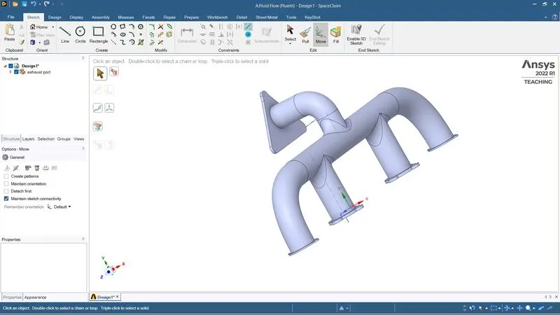
The solid and fluid volumes are combined together as a single geometry by moving to a new component.

Under workbench select the share tool to share the information between the solid and fluid volume.

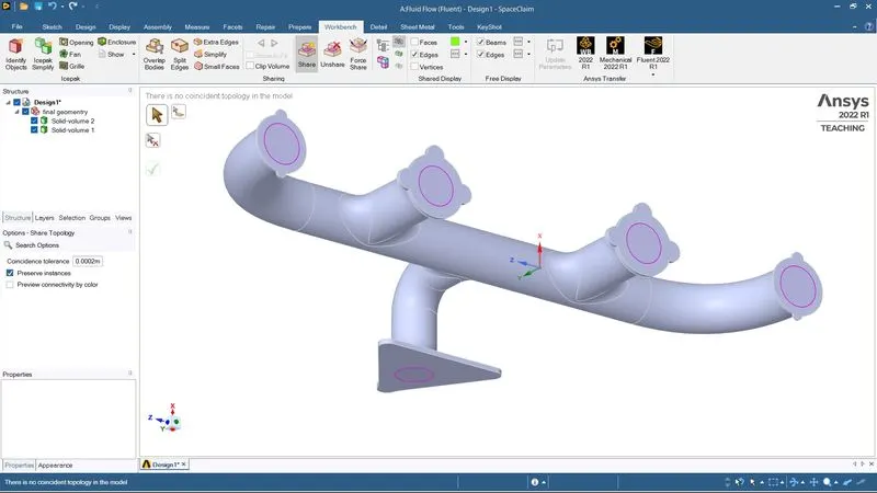
This prevents fluent from generating a non-conformal mesh.

MESHING:

NAMED SELECTION:

The boundary names are defined by using the named selection or pressing N on the keyboard. The inlet, outlet, outer wall convection, and inflation layers are the boundary names defined in the project.

MESH:

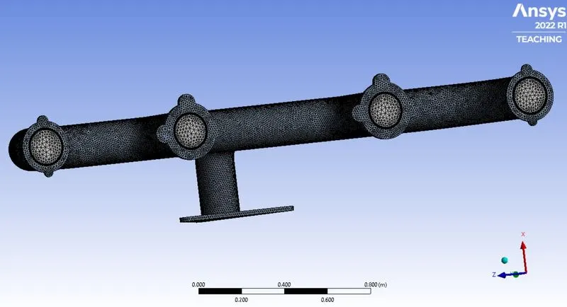
Mesh is created with the element size of 150mm with an element quality selected under mesh metric to check the quality of the mesh.

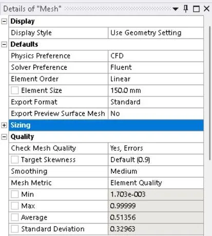
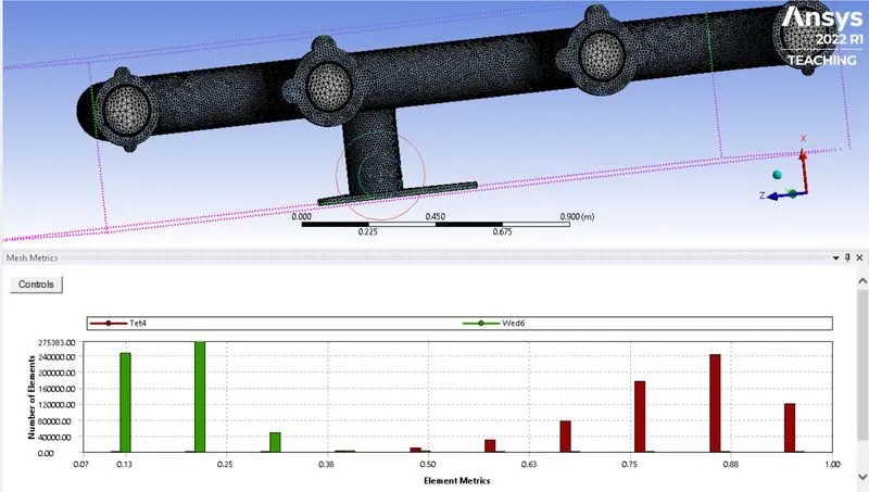
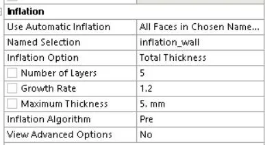
The inflation layer is created for the interior wall with 5 layers

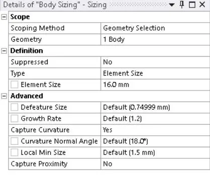
Then the body sizing is done for outer walls of 16mm and capture curvature is set to yes.

MESHED MODEL:

SETUP:

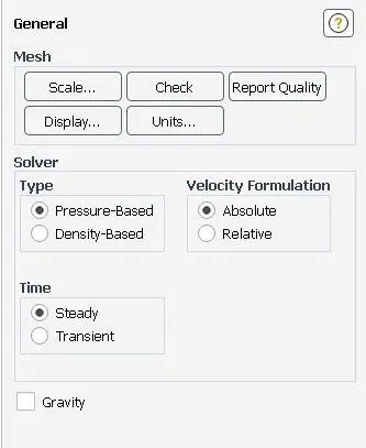
SOLVER TYPE	Pressure based
VELOCITY FORMULATION	Absolute
TIME	Steady
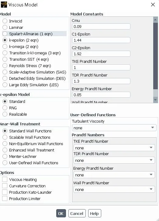
VISCOUS MODEL	k-epsilon
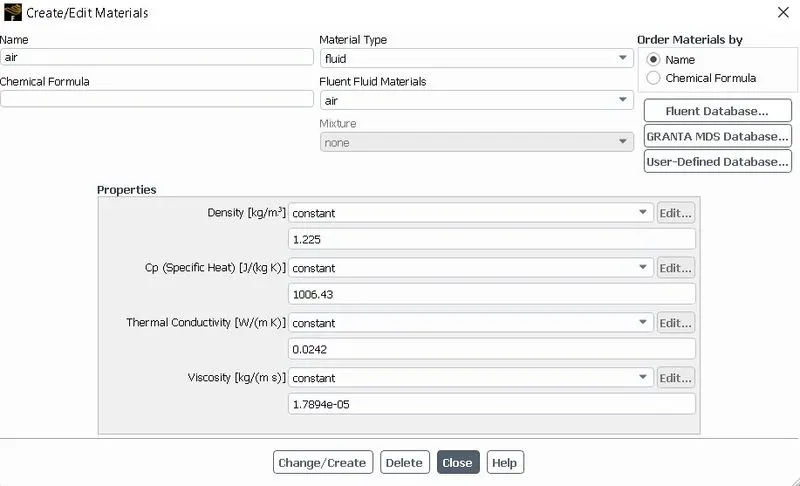
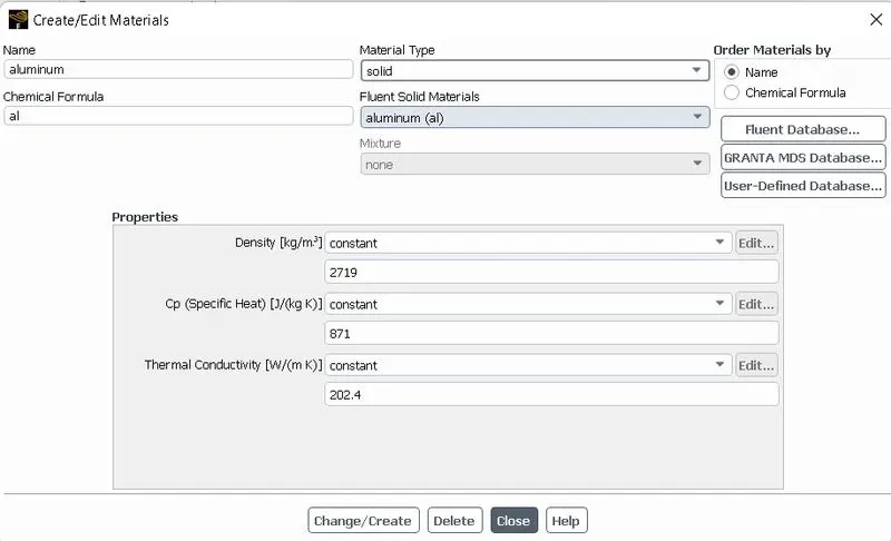
MATERIAL	Fluid – air Solid – aluminum
BOUNDARIES	INLET: Velocity inlet – 5m/s Temperature – 700k Outlet: Gauge pressure – 0 pa OUTER WALL: Convection – heat transfer coefficient – 20 w/m2k OTHER BOUNDARIES: Heat flux – 0 w/m2 [adiabatic condition]

GENERAL:

Viscous MODEL:

MATERIAL:

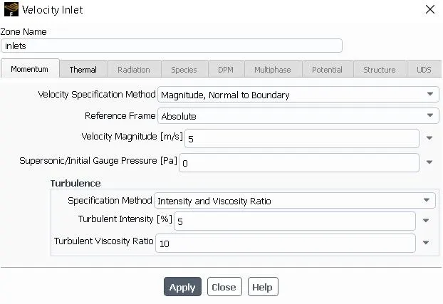
BOUNDARY CONDITION:

INLET:

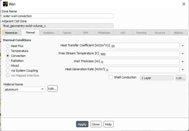
OUTER WALL:

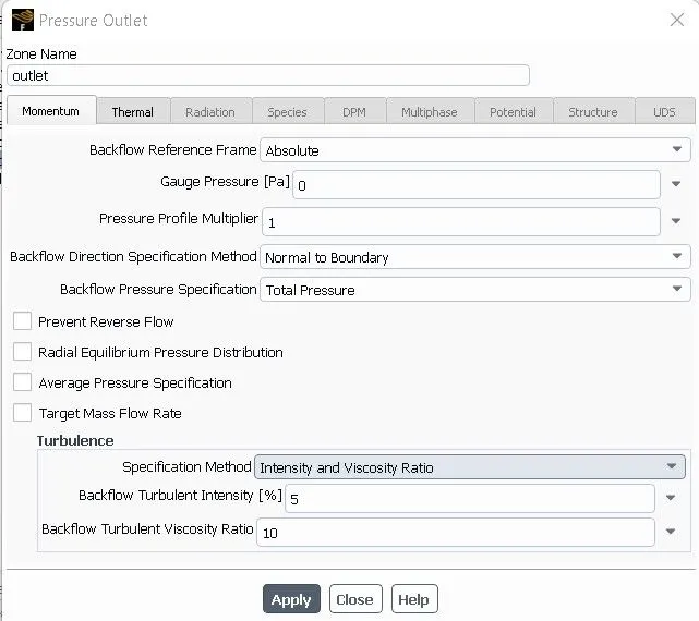
OUTLET:

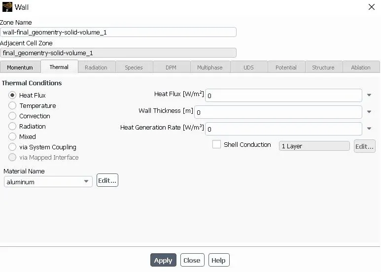
OTHER BOUNDARIES:

INITIALIZATION:

Hybrid initialization

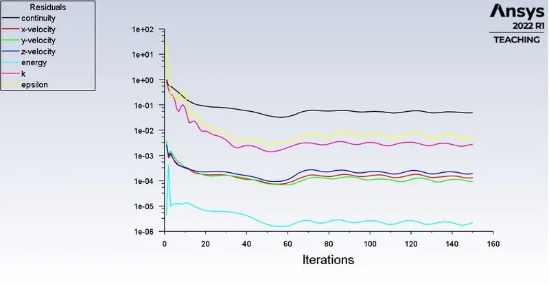
The calculation is run for 150 iterations.

RESULTS:

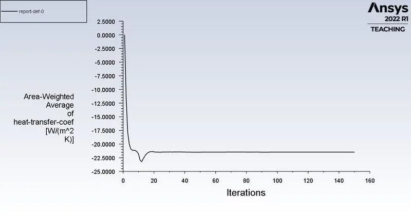
RESIDUAL:

TEMPERATURE CONTOUR:

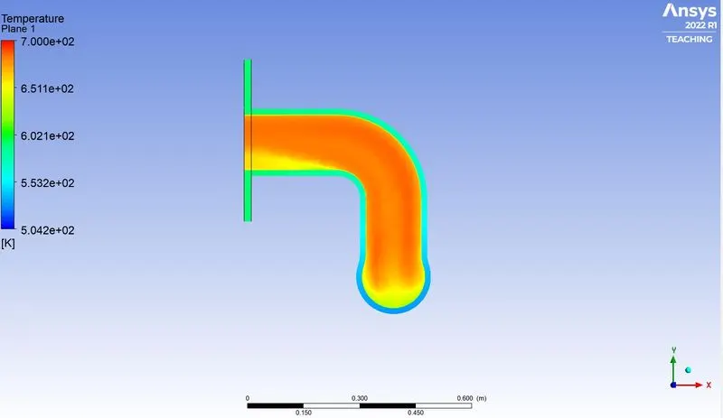
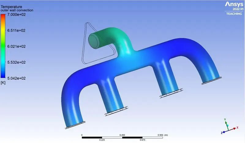
Youtube link:

https://youtu.be/Ck4bPTHcy5I

VELOCITY CONTOUR:

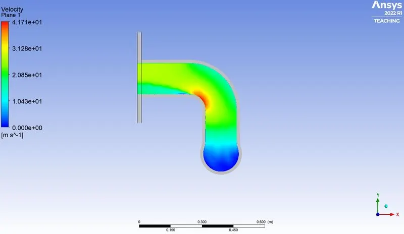
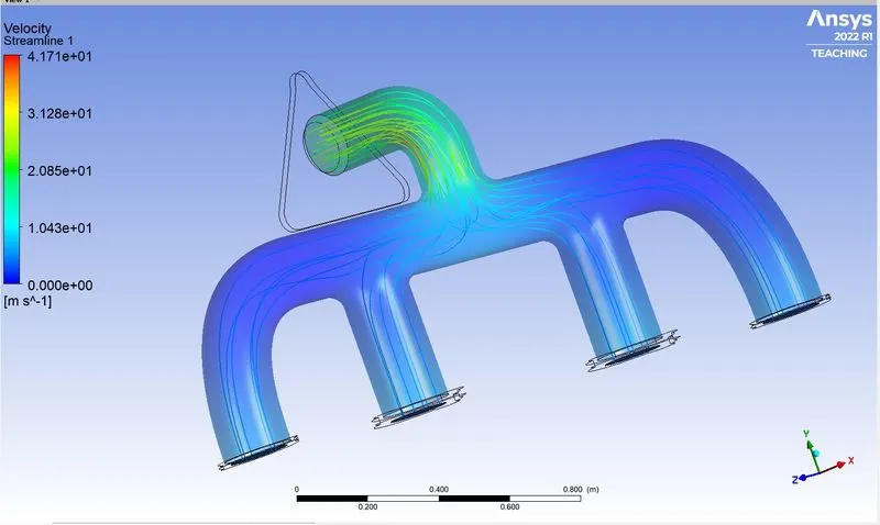
From this plot, we can say that velocity is high near the bend and is lower at the entry of the outlet

PRESSURE CONTOUR:

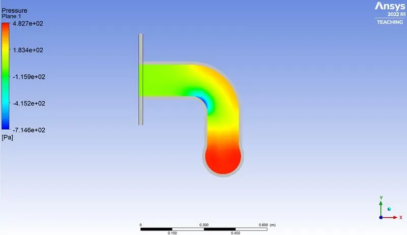
From this plot, we can say that pressure is less in the region where the velocity is high satisfying Bernoulli's principle.

TEMPERATURE STREAMLINE:

HEAT TRANSFER COEFFICIENT:

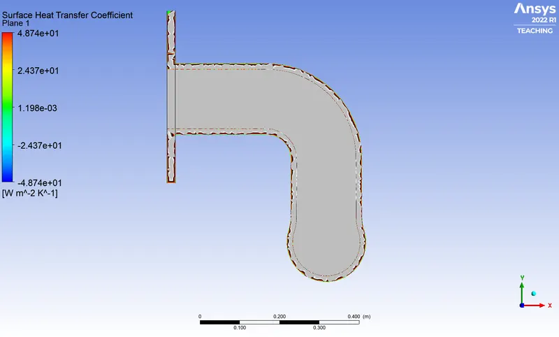
From the above plot, we can say that the heat transfer coefficient is high near the bend which is where the velocity is high.

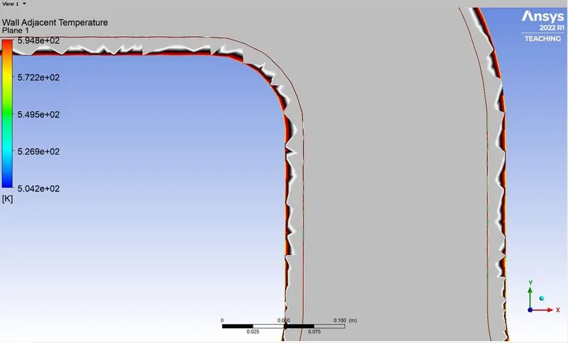
WALL ADJACENT TEMPERATURE:

How would you verify if the HTC predictions from the simulations are right? On what factors does the accuracy of the prediction depend on?

The typical flow conditions in automotive exhaust systems produce re in the range of 10^3 to 5*10^4. The exhaust flow often enters the region re<2300, especially in exhaust manifold runners. In spite of that, the flow remains actually turbulent since it has flowed through a substantial restriction. The exhaust valves and the persisting unsteady flow pulsation effects don’t favor the transition to the laminar region.

According to the sieder tate relation which correlates the Nu number with Re and Pr

Nu = 0.027Re^0.8Pr^1/3

It means Nusselt no. is the function of Reynolds no and Prandtl number

As the turbulent boundary layer in the bend of the outlet port is the thin maximum velocity of flow is observed at bend and hence higher Reynolds number.

Now, Nu = h*L/k

As the length of pipe and thermal conductivity is a constant value of h will increase as Nu increases and Nu increases as Re increases.

As per our result, the heat transfer coefficient is high for a higher value of velocity and hence our results are correct.

FACTORS AFFECTING THE QUALITY OF PREDICTION:

• More refined mesh leads to the better results
• Use inflation layers and apply boundary conditions
• Proper selection of turbulence model according to Y+ values.

CONCLUSION:

In this study, CHT analysis has done to find temperature rise at the manifold because of hot air passing through it and we predicted the heat transfer coefficient, as well as velocity contours, were created to get insight into the fluid path and maximum velocity area.

It is found that the heat transfer coefficient is more near the wall where the exhaust pipe bends.