Week 4 - CHT Analysis on Exhaust port

1.INTRODUCTION

The Conjugate Heat Transfer (CHT) analysis type allows for the simulation of heat transfer between solid and fluid domains by exchanging thermal energy at the interfaces between them. The CHT analysis of any given system is considers the physical processes and the corresponding governing equation involved for the individual subdomains separately and then correlating thier solutions by matching the required condition at the interface to get the disturbution of temperature and heat flux in coupled manner thereby eliminating the need of heat transfer coefficicent .A CHT analysis thus offers advantage of monitoring both fluid flow and heat transfer changes as well as real time prediction af wall heat transfer coefficient, temperature and velocity profiles across the domain . the conjugate heat transfer methods have become a more powerful tool for modeling and investigating nature phenomena and engineering systems in different areas ranging from aerospace and nuclear reactors to thermal goods treatment and food processing, from complex procedures in medicine to atmosphere/ocean thermal interaction in meteorology, and from relatively simple units to multistage, nonlinear processes. One such area that has gained prominence with regards to CHT analysis is in the development of an exhaust port system

The aim of this challenge is to perform steady-state simulation at an input velocity value of 5 m/s to understand the development of the velocity and temperature profiles for the given exhaust port model and to calculate the wall heat transfer coefficient on the internal solid surface

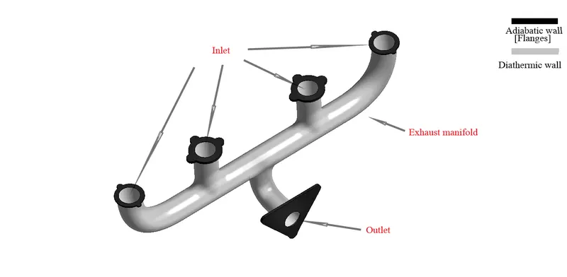
An exhaust port is essentially a construction of piping system in a configuratuion appropriate with the design requirements and constrains of the concerned application to remove or guide the burnt gases away from the combustion chamber. the given exhaust port model consists of the exhaust manifolds, collector, exhaust outlet pipe and the flanges for mounting in a four-into-one-setup

The analysis involves mesh refinement approach based on y+ value and required number of inflation layer to capture the boundary layer flow properties. The mesh study would also outline cell count, wall heat transfer coefficient values and number of iteration for convergence based on stability of behaviour of wall heat transfer coefficient values as well as some of the mesh quality attributes like like elementy qualtity, skewness, orthogonality, and aspect ratio. The result would also be validated against the analytical solution of wall heat transfer coefficient for the proposed exhaust port model configuration.

2.MODELLING

The computational domian for simulating CHT analysis of the model was done using spaceclaim which is the basic modelling software provided by ansys fluent. Since the exhaust port model has different pipe lengths in the exhaust manifold and the overall contribution from all the pipe affects the quantity and quality of discharged flow gases from the exhaust outlet pipe therefore we cannot split the geometry for simulation purpose which would result in faster computational time, Despite having isothermal bounday condition and uniform input flow with constant magnitude in all directions. In this simulation both solid volume and fluid volume will be required for discretization as wall heat transfer coefficient needs to be evaluated at the shared interface therefore it is neccesary that the solid volume and fluid volume exchange information during the solution process , And this can be enabled using share topology in spaceclaim.

2.1 MESHING

The meshing approach adopted for the given computational domain was developed to maintain the meshing quality atttributes which is , element quality ,skewness, orthogonality , and aspect ration within the range as laid out in the meshing training material of ansys outlined in the following table

Element quality	0-0.15(Bad)	0.16-1.00(Good)
Aspect ratio			Best possible value
Skewness	0-0.25(Excellent)	0.25-0.50(Very good)	0.50-0.80(Good)	0.80-0.94(Acceptable)	0.94-0.97(Bad)	0.97-1.00(Unacceptable)
Orthogonal Quality	0-0.001(Unacceptable)	0.001-0.14(Bad)	0.15-0.20(Acceptable)	0.20-0.69(Good)	0.70-0.95(Very good)	0.95-1.00(Excellent)

The reason for targeting the mesh quality which shown in the above table comes from anlysis of different types of geomerty which tells if the mesh disctretization that we have performed will develop any convergence issues during the solution process and it also helps us to locate areas in the mesh where statistcs can be improved .

2.2 CFD SIMULATION SETUP, BOUNDARY CONDITIONS, MONTITORING PLANE AND SOLUTION

The simulation on all the meshs were performed by solving RANS (Reynolds averaged navier-stokes) equation , particularly k−ε with standard wall function.

k−ε

K-epsilon (k-ε) turbulence model is the most common model used in Computational Fluid Dynamics (CFD) to simulate mean flow characteristics for turbulent flow conditions. It is a two equation model that gives a general description of turbulence by means of two transport equations (PDEs). The original impetus for the K-epsilon model was to improve the mixing-length model, as well as to find an alternative to algebraically prescribing turbulent length scales in moderate to high complexity flows.

The first transported variable is the turbulent kinetic energy (k).
The second transported variable is the rate of dissipation of turbulent kinetic energy (ε).

Near wall treatment

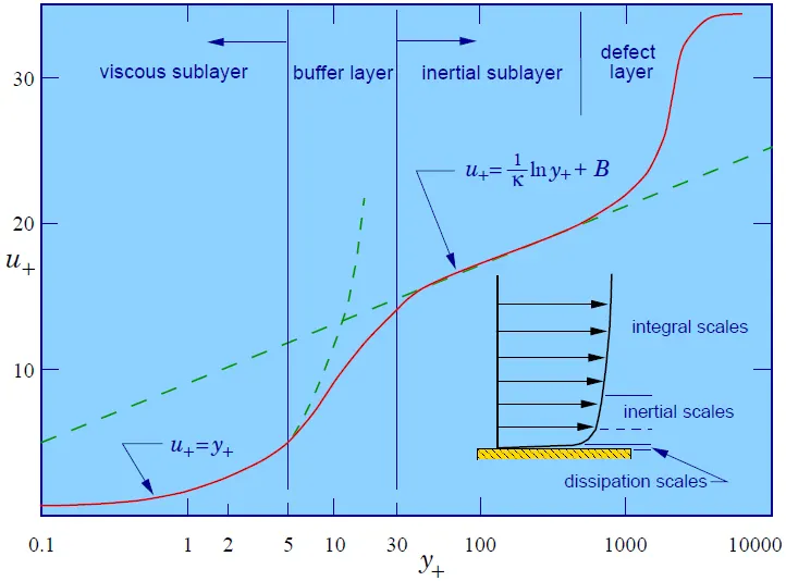
Standard wall function- As the purpose is to allow not integrating through the viscous sublayer, the lower limit of y+ is 11.225 hence standard wall function should not be used below that limit as the solution's accuracy might deteriorate in an uncontrolled manner. the flows involving seperation, reattachment and impingement where the mean flowand turbulence are subjected to pressure gradients and rapid changes, this model does not work well.

To calculate heat transfer coefficient there are two methods

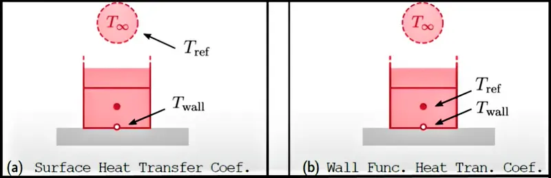
Nearest cell centroid method

using the definition of T+

T+=(Twall−Tcell)ρcpc14uk12q

where q = heat flux

and definition h with Tcell as the reference temperature we get

h=qTwall−Tcell −−−−−> h=ρcpc14uk12T+

but we can see that the Tref depends on the mesh

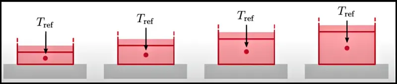
hence to capture an accurate solution we must place the cell center in y+<1 which give us a value of 1.45x10−5 m with a minimum inflation layer of 14 which puts total number of cell count to 7 million cell but due to the restriction 0f 0.5 million cell we can not solve the simulation using this method hence the better approach is to input Tref.

and to solve this simulation wall function with y+=30 was preffered to save computional time and power therefore k−ε model was used, while running the simulation double precision was enabled for all the simulation as we were computing the heat transfer coefficient from a large number of data that were being generated from the steady state simulation.

2.2.1 BOUNDARY CONDITION

For running a CFD simulation the boundary condition are very important for getting a converged solution and the boundary condition are described in the table

Named selections	Inlets	wall-fff-final_geometry_fluid-voume-fff-final_geometry_solid-volume	outer-wall-convection	wall-fff-final_geometry_solid-volume	oulet
Type	velocity-inlet	wall	wall	wall	pressure-outlet
Velocity magnitude (m/s)	5	-	-	-	-
Temperature (k)	700	-	-	-	-
Backflow temperature (k)	-	-	-	-	300
Heat transfer coefficient (W/m2K)	-	-	20(convection)	-	-
Heat flux	-	-	-	0	-
Gauge pressure	-	-	-	-	0

And the material that was used for this simulation is air which has a density of 1.225 Kg/m^3, kinamatic viscosity of 1.4207x10−5 Pa.s , Specific heat of 1006.43 J/kgK and Thermal conductivity of 0.0242 W/mK similarly, for the solid part aluminum was selected with density of 2719 kg/m^3, Specific heat of 871 J/kgK and Thermal conductivity of 202.4 W/mK

2.2.2 MONITORING PLANE

Here we are trying to find out the heat transfer coefficient of the inner wall of the pipe which varies throught out the surface in order to get a single value for heat transfer coefficient an area-weighted-average of the field has been plotted particularly surface heat transfer coefficient as the field variable and reason for doing so is explained in Near wall treatment subsection

2.2.3 SOLUTION

The nature of the CFD simulation is Steady state , The type of solver that is being used is pressure based and the reason for that is these solver are used when mach number is less then 0.3 i,e the ratio of velocity of the fluid past a boundary to the local speed of sound in the same medium(air) ,Due to the flow condition of the simulation the velocity is 5 m/s which h=gives us mach number as 0.014 which is less than 0.3

The simple scheme was imployed for solving the pressure-velocity coupling and the spatial discretization are shown in the table below

Solution method		Solution control	Relaxation factor
Gradient	Least square cell based	Pressure	0.3
Pressure	Second order	Momentum	0.7
Momentum	Second order Upwind	Density	1
Turbulent Kinetic energy	First order Upwind	Body force	1
Turbulent dissipation rate	First order Upwind	Turbulent kinetic energy	0.8
Energy	Second order Upwind	Turbuent dissapation rate	0.8
		Turbulent viscosity	1

The solution was intialised using hybrid intialization after which helped to create contour plot .

2.3 POST PROCESSING

In order to plot streamline, velocity, and temperature variation. Contour plot have been generated and the location of the plane have been provided below

Defination of plane 1

Plane Type	z distance
XY plane	0

2.4 VERIFICATION

In this numerical anlysis we have carried out the verification of solution obtained from the simulation with the analytical result in which we used k−ε equation to capture the flow

Anlytical solution

There are three different situation through which heat exchange takes place in the given exhaust manifold model. The first scenario begins with heat being conveyed from the exhaust gas to the pipe walls through forced convection during fluid flow from the inlets of the manifold to the exhaust outlet. The convected heat then travels from the internal surface of the manifold to the external surface by conduction through the solid pipe wall which is then convected the to surrounding, in this case, by natural convection as it is assumed that both the model and the air surrounding it are in stationary condition. In this numerical study, The variable of interest is the wall heat transfer coefficient on the internal surface of the pipe and Therefore, based on the boundary condition available with regards to the given model the heat transfer properties will be evaluated

Forced convection- Exchange of heat from exhaust gases to the pipe internal surface

As the reynolds number calculated for the flow suggest that the flow behaviour is turbulent in nature, The Dittus-Boelter heat transfer coefficient correlation can be used to calculate the Nusselt number which is the ratio of convective heat transfer to conductive heat transfer.

NnL=0.023.R45eD.Pnr

where D = inlet pipe diameter

Pr is the prandtl number = μ.Cpk

μ = fluid viscosity

Cp specific heat of the fluid

k = thermal conductivity of the fluid = 0.744 and

n = 0.3

The above equation is also valid for the given boundary condition based on the limitaions defined below

0.6≤Pr=0.744≤160

ReD=58189.896>10,000

(LD)>10

We know that Nusselt number is Mathematically written as Nu=hkl

where L = characteristic length

k = thermal condutivity

h = convective heat transfer coefficient .

Solving for h we get heat transfer coefficient as 19.428 Wm2K using thermal conductivity of air as 0.0242 WmK it should be noted that the Dittus-bolter heat transfer coefficient correlation was observed to be accurate in the range of ±15% and works best when the pipe surface is very smooth

BASELINE MESH

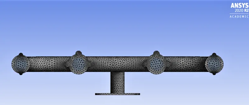
Here the mesh size was were the default value provided by the ansys meshing tool on this mesh the simulation were carried out and result are shown below

Mesh attributes

Element quality	Aspect ratio	Skewness	Orthogonal Quality
0.81966	1.8985	0.25111	0.74749

Mesh quality

Element size(max)	Nodes	Element	Heat transfer coefficient
300 mm	27496	137728	21.1906

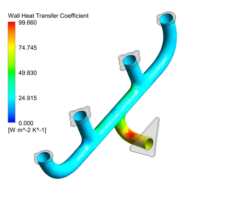
We see that the value of heat transfer coefficient from the baseline mesh is pretty close to the anlytical value which is 19.428 Wm2K.

MESH REFIENMENT

For carrying out mesh refienment we have to calculate the first cell height/thickness which was done using the below equation

y+=yurm

were

y = absolute distance

u1 = friciton velocity

μ = kinetic viscosity

For calculating ur we have to use the below equation

cf=0.0576R−15e

were

cf = skin friciton coefficient

Re = reynolds number of the fluid flow

τw=12(cfρu2)

were

u = velocity of the fluid

ρ = density of the medium

by getting these value we can find out the ur

ur=√τwρ

new mesh was generated with a y+ value of 30

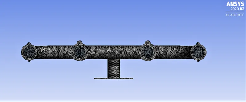
Mesh attributes (avg) with growth rate of 1.2

	Element quality	Aspect ratio	Skewness	Orthogonal quality	First cell thickness	number of inflation layer
Refined Mesh	0.74299	3.8072	0.21373	0.78432	0.88mm	3

Mesh quality

Body sizing (solid)	Body sizing (fluid)	Nodes	Element	Heat transfer coefficient (Simple solver)	Heat transfer coefficient (Simplec solver)	Heat transfer coefficient (coupled solver)
19 mm	13 mm	761977	492254	21.384775	21.386341	21.389282

We can see that the mesh attributes lies between the recommended value as shown in MESHING section above therefore the solution is going to converge

2.5 CONVERGENCE LEVEL

Three different scheme i,e SIMPLE,SIMPLEC and COUPLED were compared with regards to convergence study. Simple scheme is iterative in nature , robust and is quicker per iteration than other pressure based solver. SIMPLEC scheme, similar to SIMPLE scheme, allows increased under relaxation to the pressure correction term that improves in convergence times especially when employed in complicated flows with turbulence and/or supplementry physical models and as such offers greater diversity in terms of computational problems for implementation over SIMPLE scheme. While SIMPLE and SIMPLEC schemes are segregated types of schemes i.e., pressure and velocity terms are updated sequentially, the COUPLED scheme on the other hand updates the pressure and velocity terms simultaneously. this allows the COUPLED scheme to be more efficient in its single phase implementation especially for steady state flows offering superior performance over the segregated algorithms thereby requiring fewer iteration to converge. the selection of scheme for different terms spatial discretization includes assigning gradient to least square cell based scheme, pressure to second order scheme, momentum to second order upwind scheme, turbulent kinetic energy to first order upwind scheme and turbulent dissapation rate to first order upwind scheme of which the turbulent kinetic energy and turbulent dissapation rate. Least square scheme is the default gradient method chosen by ANSYS Fluent which is used to compute the changes the values across the centroid of two cells along the vector path and is a computationaly less expensive scheme offering comparable accuracy to the node based gradient scheme, both of which are superior to cell based gradient scheme. The second order scheme for the pressure makes use of the central differencing scheme and is generally considered to be more accurate than the standard and linear schemes as well as robust in the case of skewed meshes.A second order upwind scheme is choosen for the momentum and energy term that makes use of the quantities at the cell faces values to compute a cell-centered solution at the cell centroid leading to a second order accurate solution. turbulent terms viz., turbulent kinetic energy and turbulent Dissaption rate are set at first order upwind scheme by default which makes use of quantities at the cell faces as the cell-averages value indicating that it is first order accurate. The reason to have the turbulence terms discretised using the first order upwind scheme is based on observation from simulation across different application when using a higher or even second oeder upwind scheme leads the computational cost to become more expensive (more compute time) solution while also demonstrate stability issue in the form of repeating oscillation of values and not necessarily guaranting always a more accurate solution. Convergence criteria option was checked off, however, the residual values which measures the local imbalence of conserved variable in each control volume such as continuity , x-velocity, y-velocity, z-velocity ,k-ε and energy were monitored throughout the solution process for the defined number of iteration to allow the actual behaviour to be developed i.e., the formulation of a fully developed flow profile and consistent rate of heat transfer along the interface between the solid body and the fluid volume.

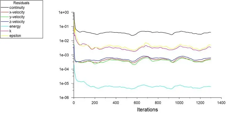
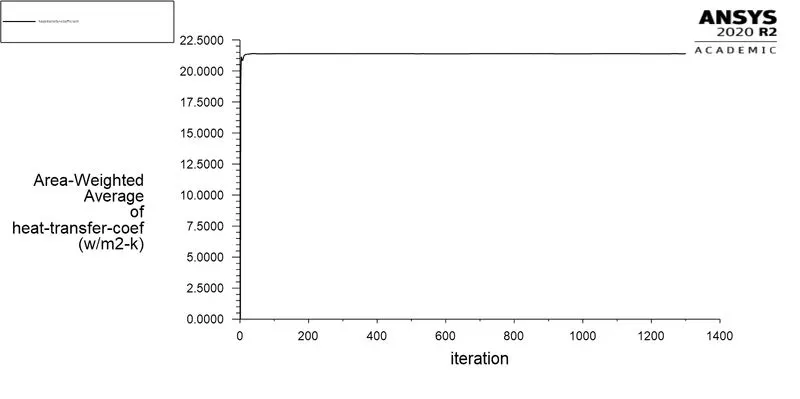
Residual and Heat transfer coefficient plot for refined mesh using k−ε turbulence model with SIMPLE solver

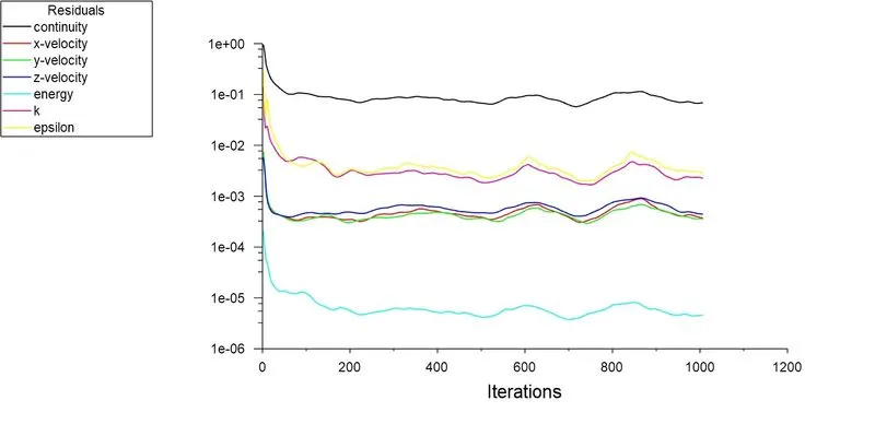
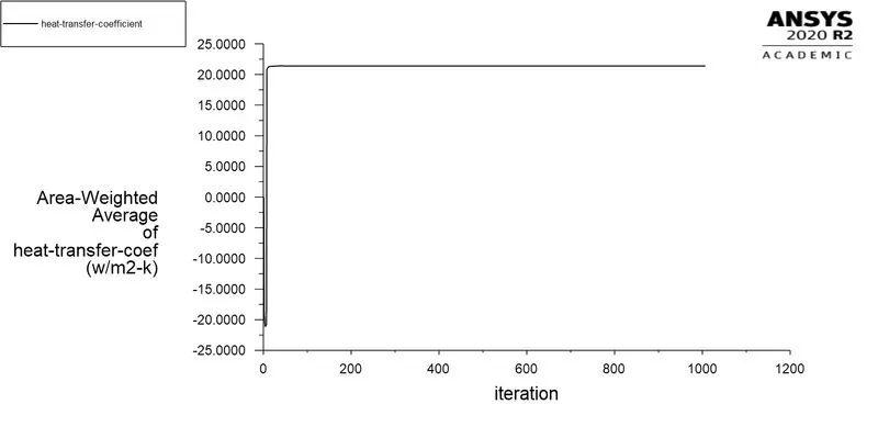
Residual and Heat transfer coefficient plot for refined mesh using k−ε turbulence model with SIMPLEC solver

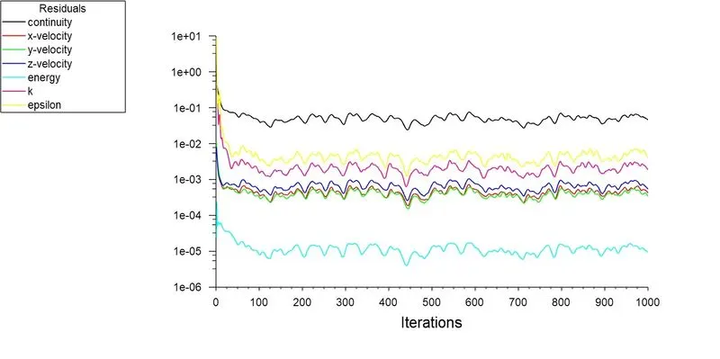
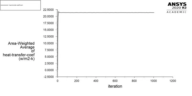
Residual and Heat transfer coefficient plot for refined mesh using k−ε turbulence model with COUPLED solver

The residual plot obtained from the SIMPLE scheme looks more stable then the residual plot obtained from SIMPLEC and COUPLED scheme solver Therefore, the heat transfer coefficient obtained from SIMPLE scheme is more realiable hence the result of the same is displayed it the result section

RESULT :

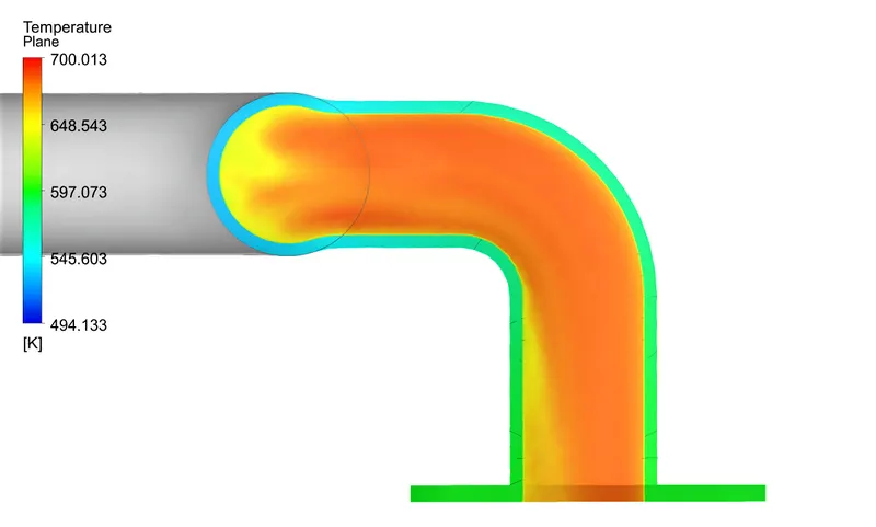
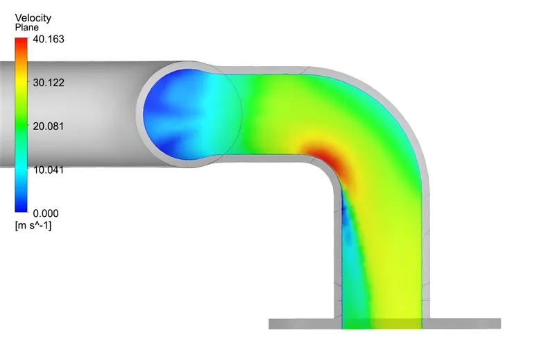
Temperature and velocity contour plot at the exhaust oulet

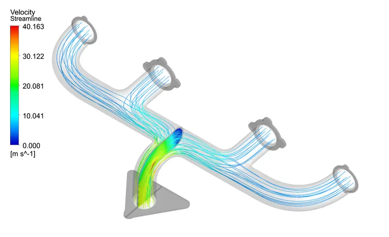
Plot showing Velocity streamline from inlet to outlet of the exhaust port

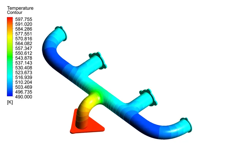
Temperature diturbution over the solid surface is shown using contour plot

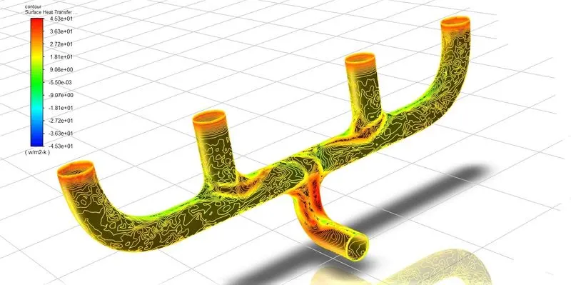
Surface heat transfer coefficient over the inner surface of the solid pipe is shown using contour plot ( with counter line)

Numerical solution of heat transfer coefficient	Analytical solution of heat transfer coefficient	Error
21.384775 Wm2K	19.428 Wm2K	10.07%

As seen the numerical computed value overpredicts the heat transfer coefficient by 10.07% when compared with analytical solution obtained from Dittus-boelter heat transfer coefficient correlation. It should be however noted that the numerical computed value is an average value while the analytical solution of heat transfer coefficient holds good for a straight sectioned pipe with fully developed flow profile throughout the pipe. There are other correlation available to compute heat transfer coefficient which can be used. But better approach would be to perform an experiment or interpolate the value of heat transfer coefficient from previously conducted experiments