Week 4 - CHT Analysis on Exhaust port

Objective:

The aim is to perform the simulation on exhaust port to analyse the conjugate heat transfer (CHT).

Conjugate Heat Transfer:

It is mathematically stated problem, describes the heat transfer between a body and a fluid flowing over or inside it as a result of the interaction of two objects. The physical processes and solutions of the governing equations are considered separately for each object in two subdomains (Body & Fluid domain). Matching conditions for these solutions at the interface provide the distributions of temperature and heat flux along the body–flow interface, eliminating the need for a heat transfer coefficient. Moreover, it may be calculated using these data.

The best way to analyse the solution for it is by using Numerical method. Set the boundary conditions for both the interface, process and converge the solution.

Application:

Conjugate heat transfer methods have become a more powerful tool for modelling and investigating nature phenomena and engineering systems in different areas ranging from aerospace and nuclear reactors to thermal goods treatment and food processing, from complex procedures in medicine to atmosphere/ocean thermal interaction in meteorology.

• Heat Exchangers and Finned Surfaces (e.g., IC engine, heat sink, car radiator)
• Thermal Treatment and Cooling Systems (e.g., thermal depolymerisation, cooling tower)
• Simulation of Industrial Processes (e.g., inline four engine exhaust port)
• Technology Processes (e.g., graphics card)

Efficiently combining heat transfer in fluids and solids is the key to designing effective coolers, heaters, or heat exchangers. The fluid usually plays the role of energy carrier on large distances. Forced convection is the most common way to achieve high heat transfer rate.

In some applications, the performances are further improved by combining convection with phase change (for example liquid water to vapour phase change). Even so, solids are also needed, in particular to separate fluids in a heat exchanger so that fluids exchange energy without being mixed.

Solving & modelling approach:

• Import the inline four engine exhaust port geometry in space claim.
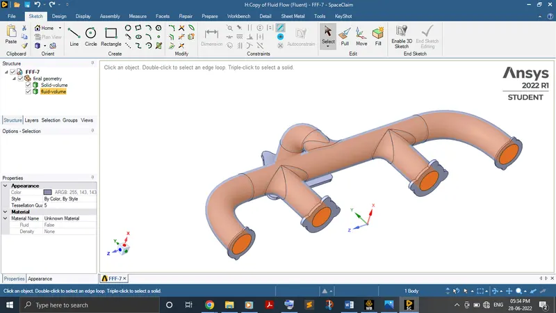
• CHT analysis requires solid and fluid volume. So, in space claim use volume extract option to create fluid volume.
• Move these individual volume into single component.
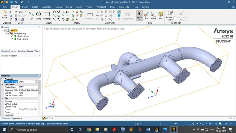
• Set the share topology from none to share to share the information between two volume interfaces.
• Load the geometry in meshing. Do the named selections for the inlets, outlet & convection outer wall faces and mesh the geometry for baseline stuff. To analyse further, refine mesh.
• Do the necessary physics and boundary conditions setup in setup to converge the solution.
• Finally, compare the result of contour and graph plot.

Pre-processing and solver setting:

Baseline mesh:

Geometry:

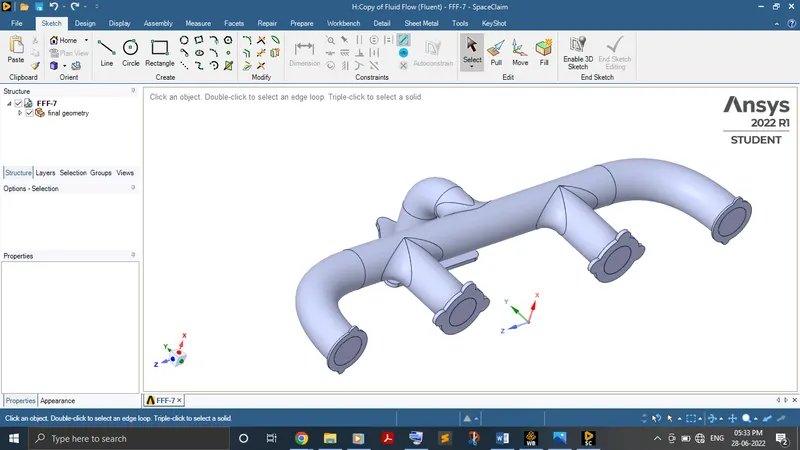
Import the geometry in space claim.

Use volume extract option to create fluid volume.

Set the share topology from none to share to share the information between two volume interfaces.

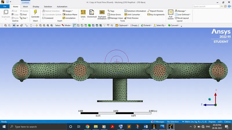
Meshing:

Load the geometry in meshing and do the named selections.

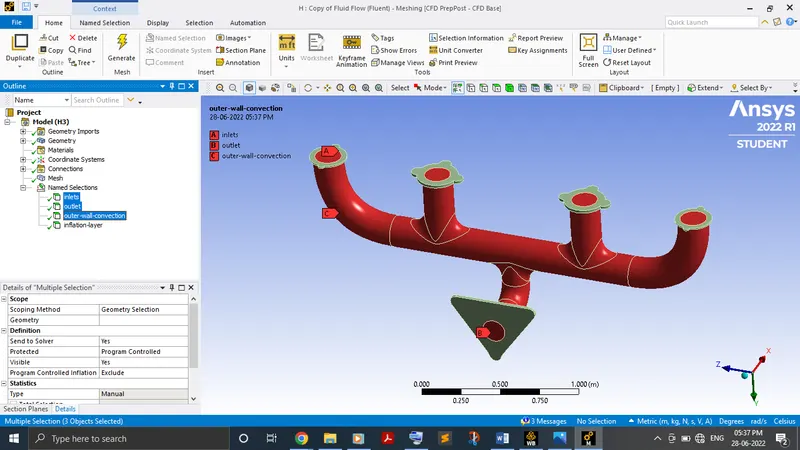
Do the baseline mesh for the geometry.

Setup:

Solver type - Steady state pressure based

Model - Energy equation, K-epsilon viscous turbulence model

Material - Fluid (air), Solid (aluminium)

Boundary conditions:

• Inlet velocity - Velocity magnitude (5 m/s), Temperature (700 K)
• Outlet pressure gauge - 0
• Outer wall convection - Thermal condition (convection, Heat transfer co-efficient (20 W/m²K)

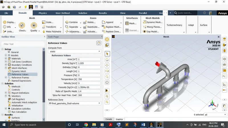
Reference values:

Results:

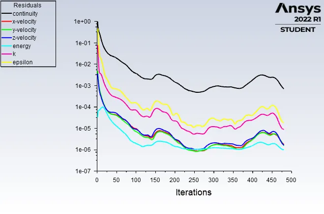
Residual plot:

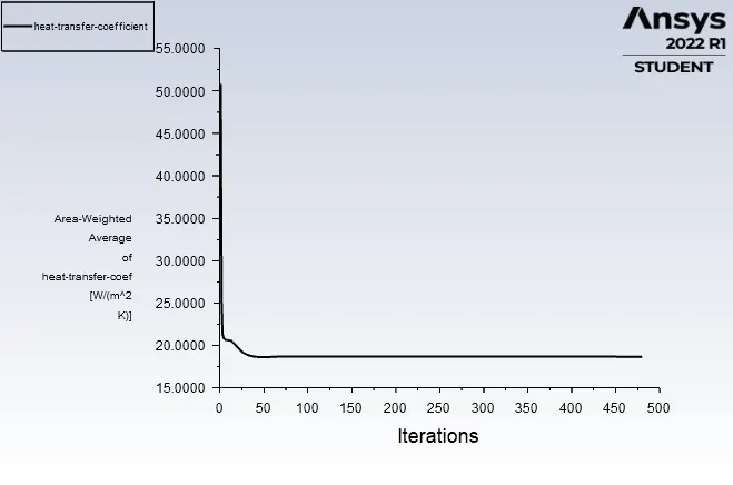
Surface heat transfer co-efficient: 18.68539 W/m²K

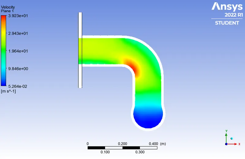
Velocity contour:

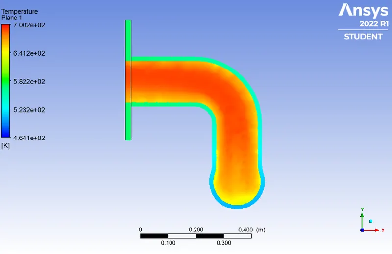
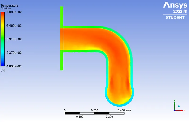
Temperature contour:

Refinement 1:

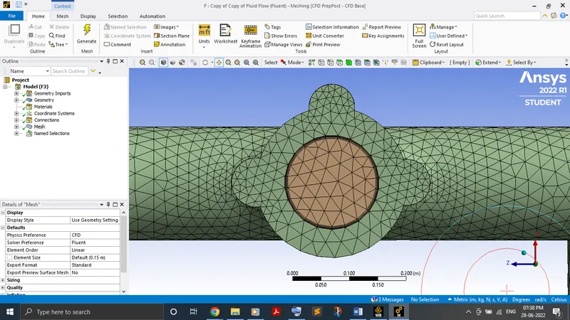
Mesh update:

Solid volume body sizing: 0.75 m

Inflation layer: 5

Inflation method: Total thickness

Setup update:

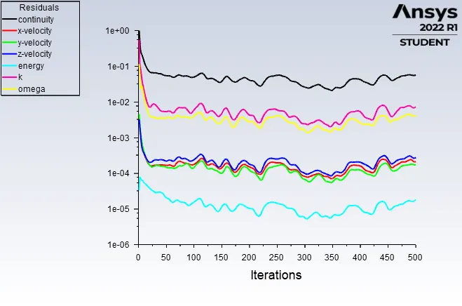
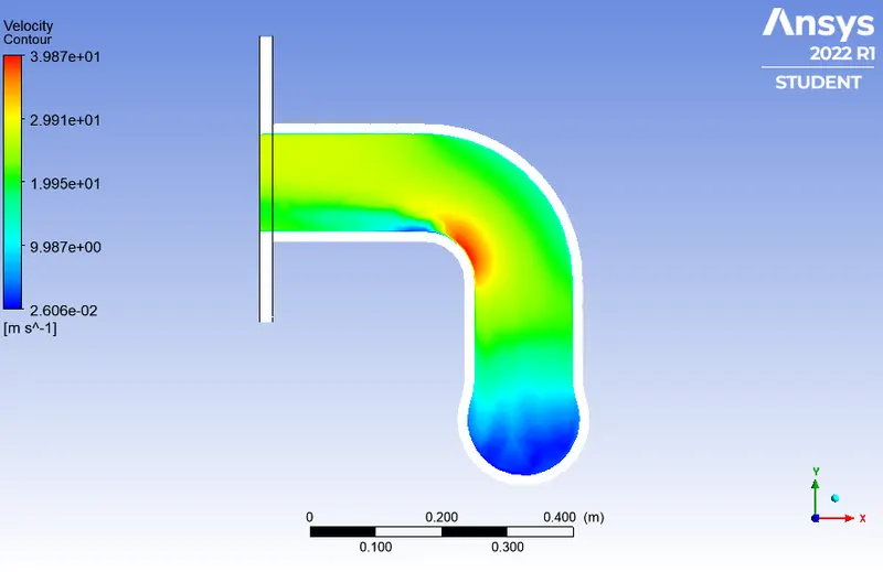
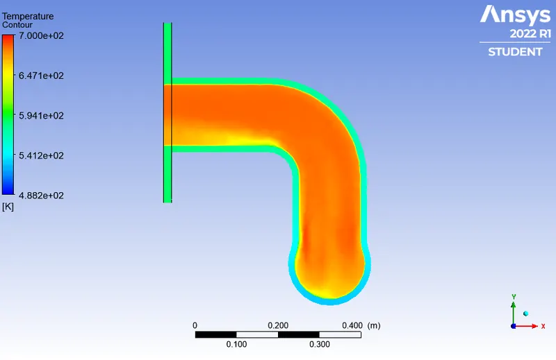
Viscous model - K-omega turbulence model

Results:

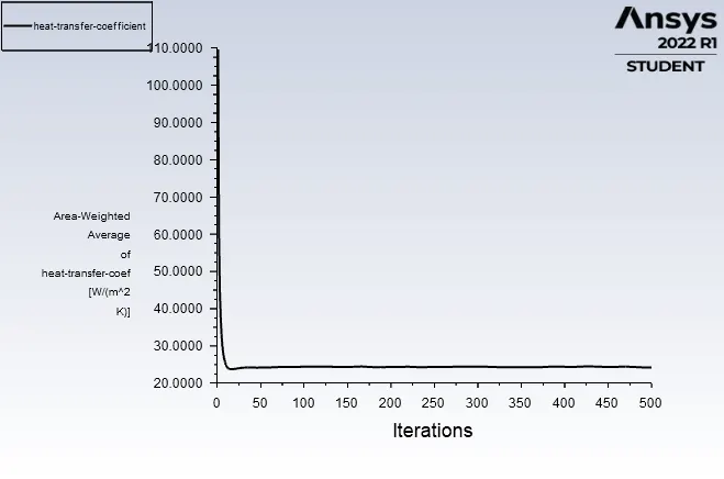
Residual plot:

Surface heat transfer co-efficient: 24.229425 W/m²K

Velocity contour:

Temperature contour:

Refinement 2:

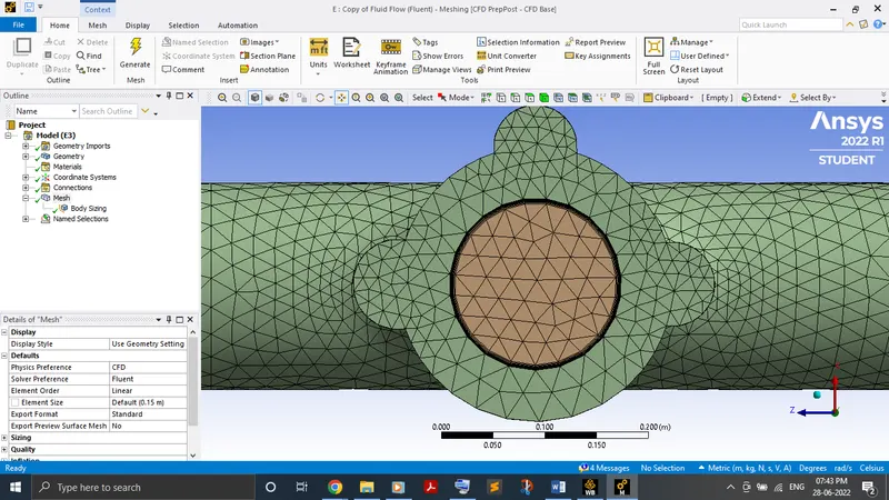
Mesh update:

Solid volume body sizing: 0.5 m

Inflation layer: 10

Results:

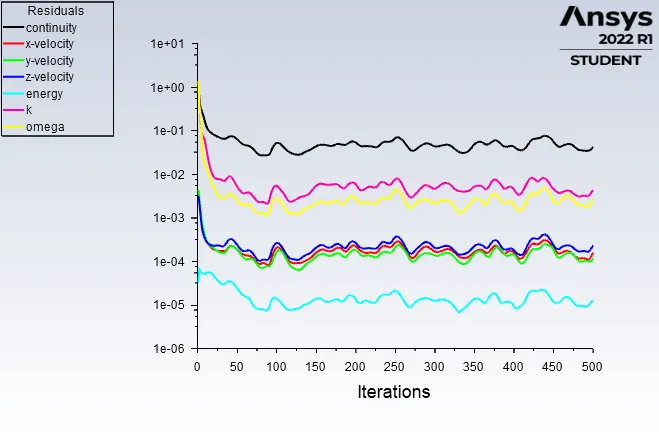
Residual plot:

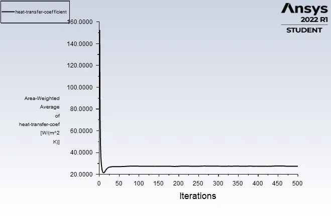
Surface heat transfer co-efficient: 27.3517 W/m²K

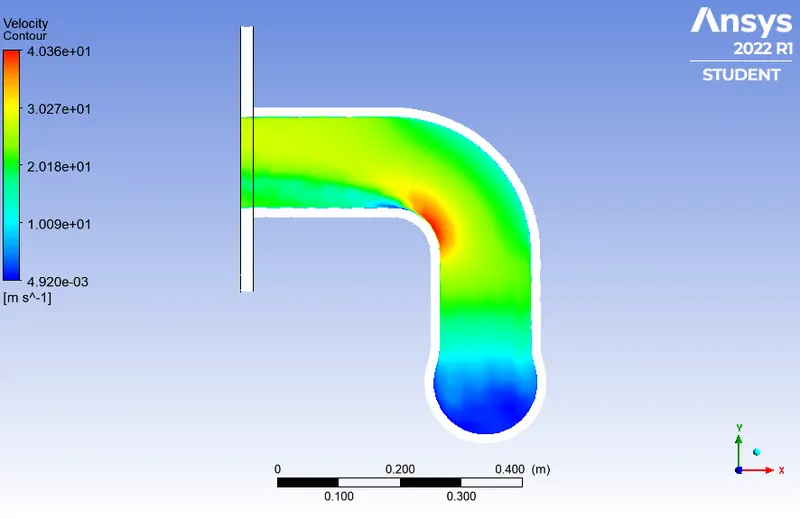
Velocity contour:

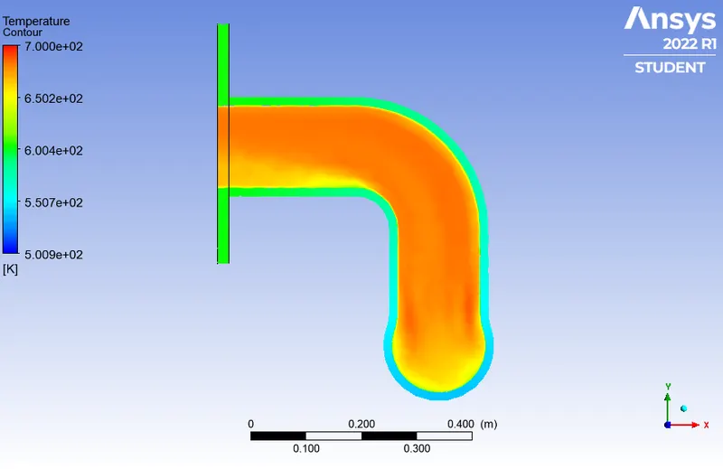
Temperature contour:

Refinement 3:

Mesh update:

Solid volume body sizing: 0.25 m

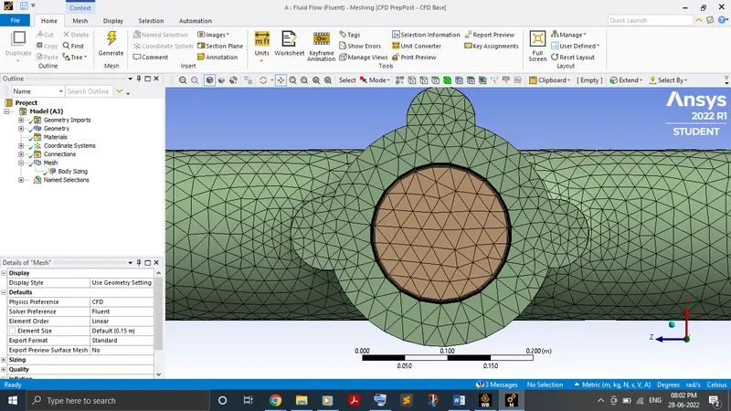
Results:

Residual plot:

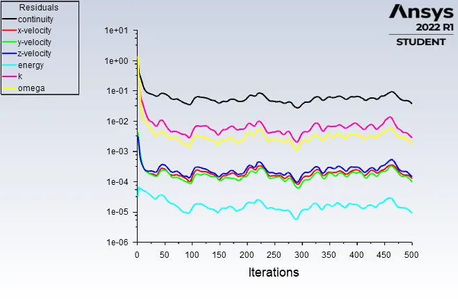
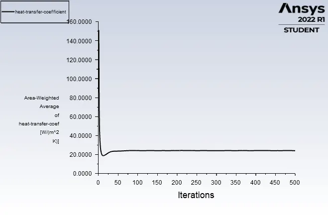
Surface heat transfer co-efficient: 27.549108 W/m²K

Velocity contour:

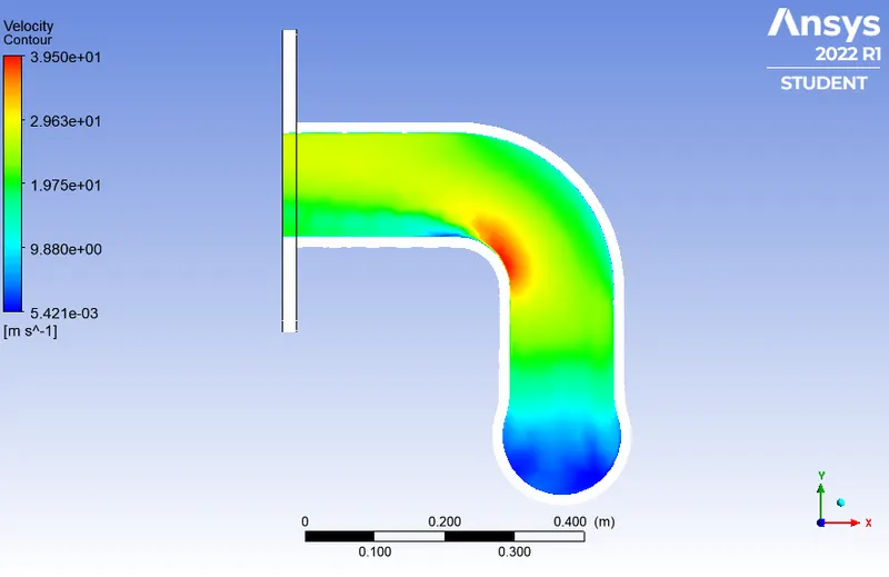
Temperature contour:

Refinement 4:

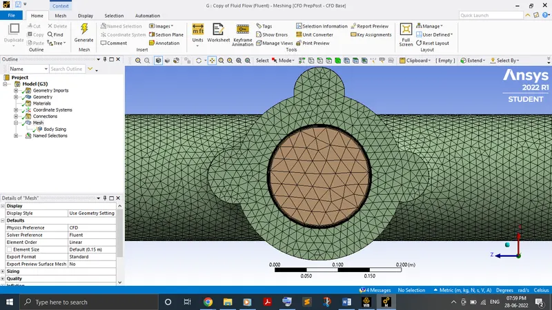
Mesh update:

Solid volume body sizing: 0.12 m

Results:

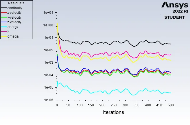
Residual plot:

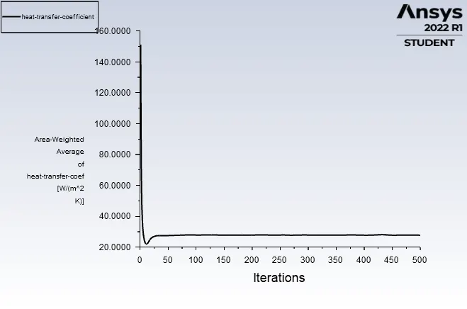
Surface heat transfer co-efficient: 27.843131 W/m²K

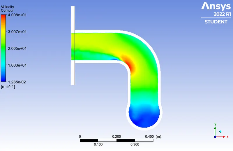
Velocity contour:

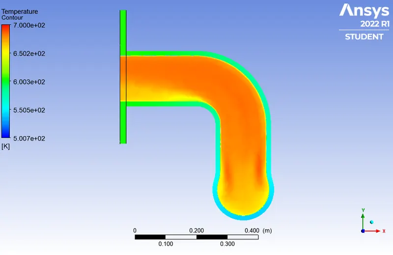
Temperature contour:

Conclusion:

From the result obtained, we can conclude that the HTC starts to increase at walls. To verify it, we refined the geometry much finer. The accuracy is completely depends on maintaining Y+ value and turbulance model. Generally, if we want something to cool efficiently, we need high HTC and vice versa if we need to insulate. So, in our case high HTC is required and that's what we obtain as result as well.