Week 4 - CHT Analysis on Exhaust port

CONJUGATE HEAT TRANSFER:

The type of heat transfer corresponding to the combination of the heat transfer in solids and heat transfer in fluids. Heat transfer in solid called as conduction and heat transfer in fluids is called convection.

Conduction occurs due to the direct molecular collision. The faster kinetic energy collides with the low-speed kinetic energy and heat transfer occur.

Convection process is not happend alone. It combined with the conduction or radiation.

(CONDUCTION + ADVECTION = CONVECTION).

So, the conjugate heat transfer occurred mostly in the cooling process like HEAT SINK, BATTERY COOLING, AIRFLOW OVER THE SOLID OBJECT FOR COOLING.

Whenever the solid and fluid interface appears, this type of CHT analysis can be done to find the optimum results by using the Ansys. It allows the simulation of the heat transfer between solid and fluid domains by exchanging the thermal energy at the interface between them.

CHT ANALYSIS ON A MODEL OF AN EXHAUST PORT:

Here we use the inline four cylinder engine exhaust manifold, where the conjugate heat transfer is analyzed to find the optimum heat transfer coefficient. Fluid volume is extracted from th the port and consider as the fluid region where the air enters into the region. Since it has the interface of the solid and fluid domain so this type is called as CHt analysis.

When we generate the baselien mesh, the non-conformal mesh is generated which affect the results. To make a conformal mesh share topology option is used which make the perfect mesh.

SETUP :

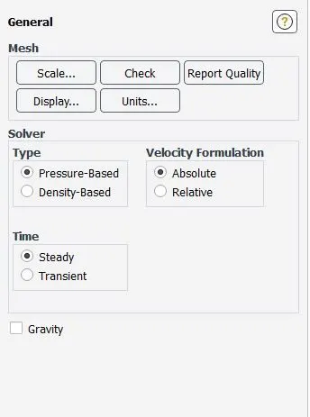
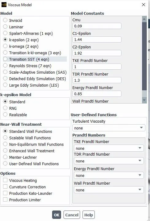
Pressure based solver is used for the analysis. Steady state and enable the energy to measure the temperature. The Turbulent k-epsilon method is used to run the analysis.

BOUNDARY CONDITION:

Material - air

Inlet - velocity inlet - 5m/s , temperature - 700k

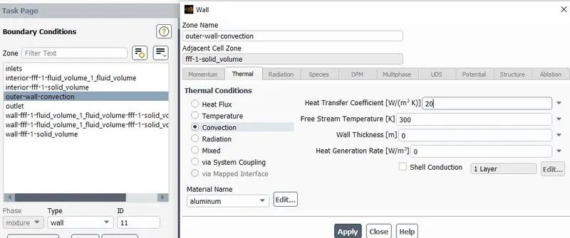
The outer wall of the port - convection, Heat Transfer coefficient - 20w/m^2k.

Free steam temperature - 300 k.

Outlet - Pressure oulet.

Use the hybrid initialization and run the analysis to get the result.

let's start with the Fluid fluent model in workbench

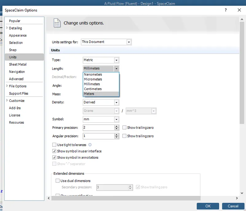
Lets double click on the "Geometry" to open the spaceclaim, once spaceclaim has launched i am going to change units first to meters.

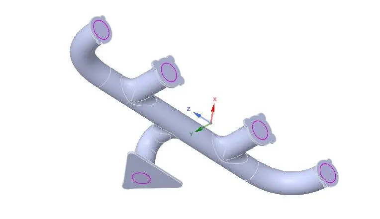
Now i am going to import the geometry. This is made up geometry but it contains all the features that actually exhaust port can have. our objective is to basically simulate the flow through it and it exchange the heat with solid.

We assume that the fluid which is coming through the exhaust basicaly all these 4 inlets and we assume that the fluid is very hard and it heat the solid pipe from inside

and on the external surface we are assuming that there is particular heat transfer coefficient and in the real world scenario the engine is air cold meaning it explose to air and air has particular heat transfer coefficient and that could be provided as the input , that typically depends upon the Reynolds number of the external air.

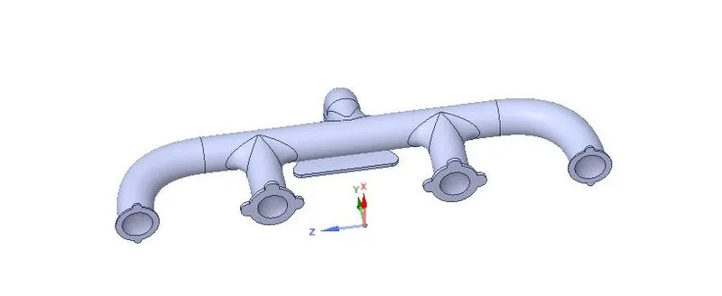
I need to add additional enclosure just like the external flow simulation, but in this case i am not going to do that we are just going to say that for the outer boundaries we need to specify that there is a particular value of heat transfer coefficient and that's going to determine heat-transfer.

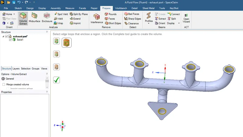
The first step is to extract the fluid volume , i am going to select the select edge option and select the 5 edges of this component here is see

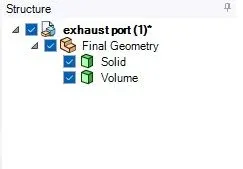
Move volume and solid component to a Final Geometry folder

Then i am going to do shared Topology for this i went to 'Workbench --> SharePrep and i can see below the picture is coming out and pink circles indicates this. basically this step taking care of the interfaces so that u just one interface between in our solid block and our fluid block.

In the meshing part i am going to generate the mesh first of all.

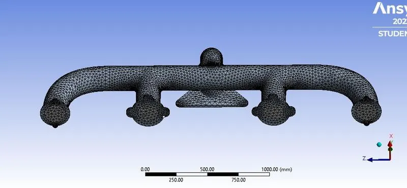
when i am zoom this component then i can see that the volume and solid parts are kind of separate or i have non-conformal mesh or u can say physical gap between the two bodies.

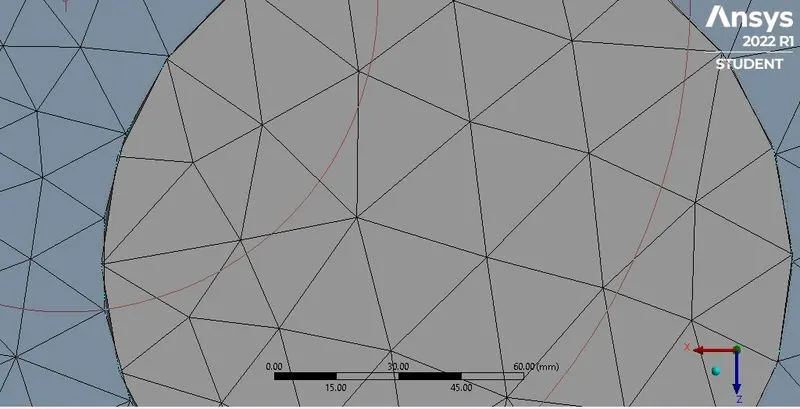
so for conjugate heat transfers simulation we need to overlap its perfectly. so i order to do that i need to do something called sharred apology.

so let me close the meshing and go back to workbench and reset the meshing and go back to Spaceclaim and here go to properties and enable shared apology

this actually help us to make the mesh clearly.

first of all take two volume and click on those two volumes and then right click and move into a new component and this is our basically a 'final geometry'

Let's click on FFF and deleted the empty components. Now go to 'workbench' and click on 'Shareprep' , basically this step take care of the interfaces so that we have one interface between solid block and fluid block and see can see pink circles in the holes and these telling us where the information is shared.

so let go to meshing part again, Now create a mesh now we can see that the meshing part is perfectly fine.

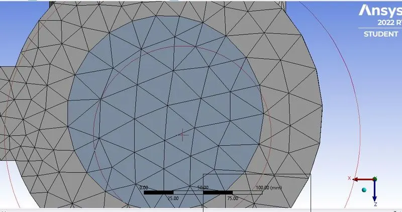
Remember once we created a general baseline mesh just go ahead and delete it.

well the question is why i am doing this. because i dont created any named surfaces here. Generally we have to created a named and then generated a mesh.

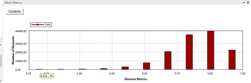
So , i created a name selection inlet, outlet and outer-wall-convection and then created a mesh so here as i can see that i have 138238 elements cells which are very less as prospective of academic cells (half-milliion).

so lets looking at the element quality we want minimum of 10% of this particular case but here i got 22% which is perfectly fine.

Now, let's jumping to the setup part i am gong to be using here pressure based Solver with the steady state condition.

so for the set-up physics but im solving energy equation here with the k-epsilon model

For the material, in case of fluid we are using air and for solid, we are going to use aluminium.

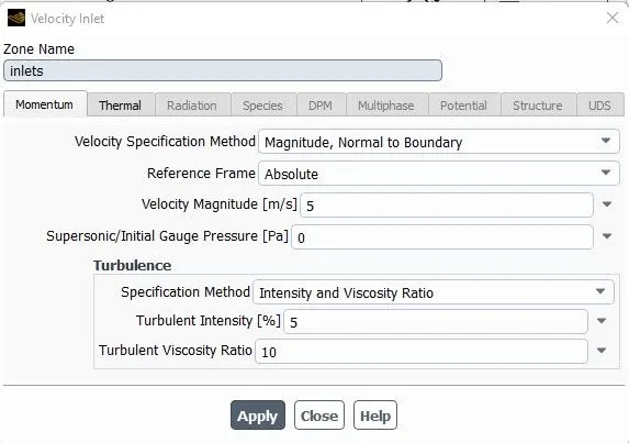
For boundaries,i am using inlet velocity @5m/s and temperature is 700k

Velocity inlet

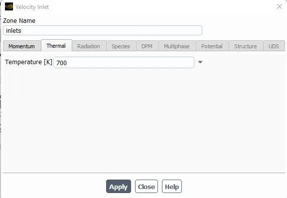
Now i am going to give the name that i have set up the component that we give the name and provide such value of heat transfer coefficient {20w/m^2-k} this value is coming from the experimental data.

Wall

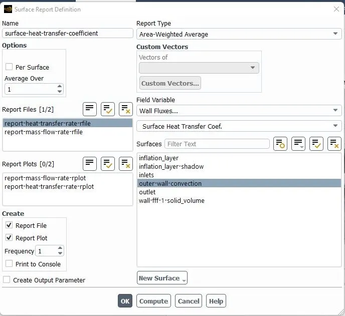
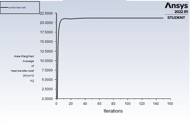
Now, i am going to make a surface report for Surface-heat-transfer-coefficient

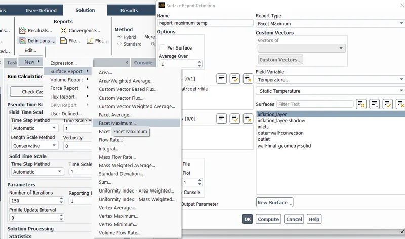
Let's find out the value of maximum temperature

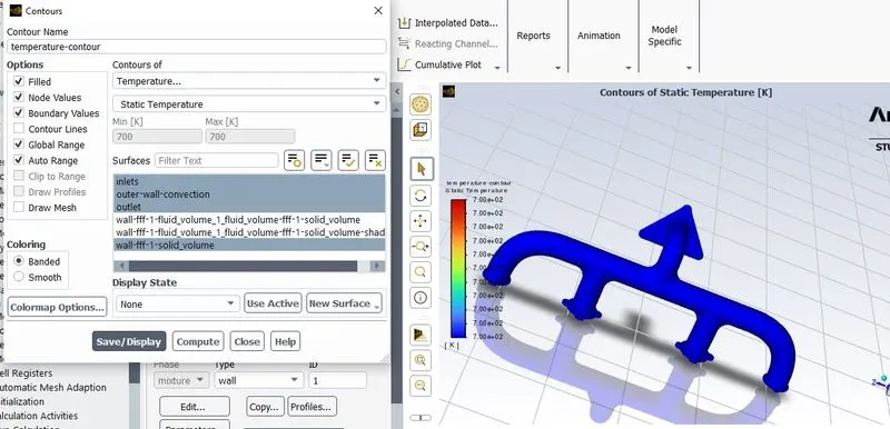
Now go to solution and initialize the case using hybrid initialization and make contour plot as shown below.

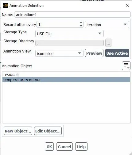
Create a solution animation , this animation could be created each and every iteration

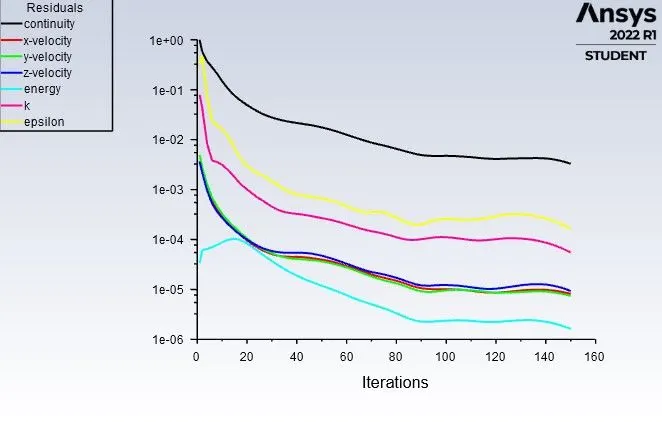
So now let's RUN the simulation for 150 iteration and gets some of the results like residuals.

Results of Case 1:

Mesh size : 150 mm

Solver: k-epsilon for baseline mesh

Surface Heat transfer coeff.

so in order to find the surface heat coef. i should need to go back to meshing part and here firstly i want to hide the solid component by going to

Geometry -- > Final geometry---> Solid and right click here to hide the solid component and whatever the left component is left that is basically is called liquid component and double click on it and press the shortcut key 'N' to create a name ass 'inflation layer'. Inflation layer is basically called as the surface between solid and liquid body. so back to Ansys Fluent and do the simulation.

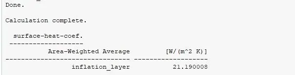
So in the postprocessing , first of all in the solid volume enable the outer wall.

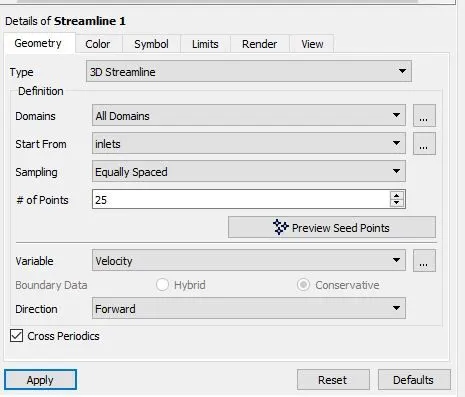
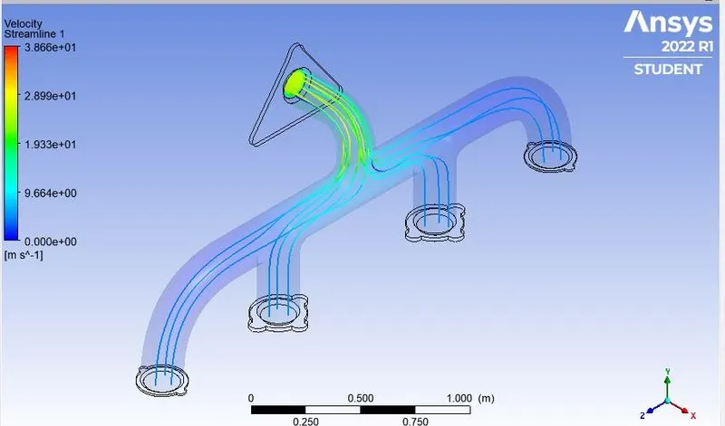
Now, create a streamlines and start streamline with inlet and after applying all the inputs we can clearly seen high & low velocities in the ports

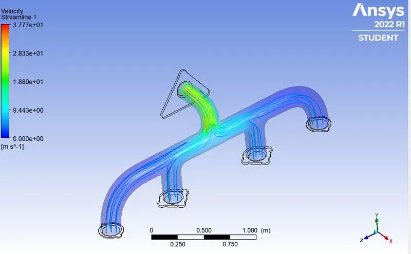
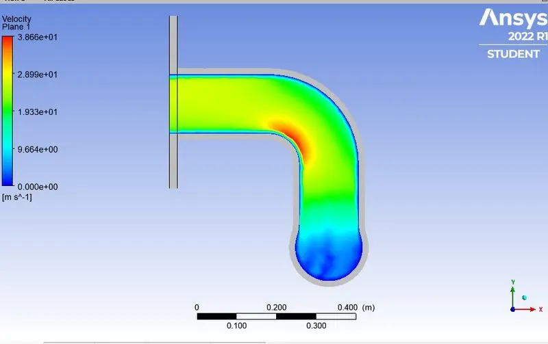
The velocity in the all inlet's preety much same and velocity at outlet is very very high s o due to higher velocity we have higher Reynold's number there which mean we have a higher heat transfer coefficient there means there could be more heat transfer from the fluid to the solidso that's why the temperature of that solid's location is higher.

Now, insert a plan and evaluate the temperature and velocity contours

Velocity contour

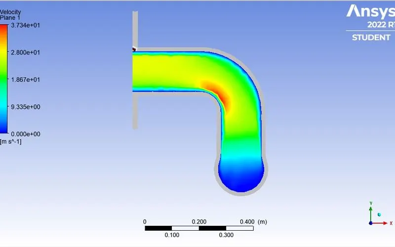
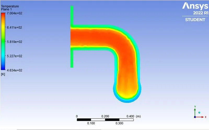
Temperature contour

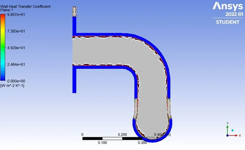
Wall Heat transfer coeff.

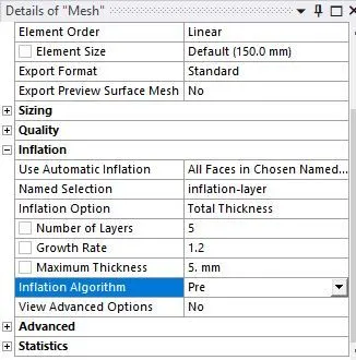
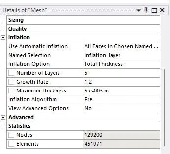
Refined case : In this case the mesh is finer at the solid part, having elements of about 451971. Also 5 inflation layers are provided with a growth rate of 1.2 and maximum thickness of 5e-003m.

Go to meshing part and click on inflation and here we choose 'smooth transition ' and hide the upper body of exhaust port and go to face selection and select the body part and provide the name as 'inflation-layer' by cliking the shortcut key 'N'

and do some changes in the mesh as per given below :

and we can see that inflation layer got created.

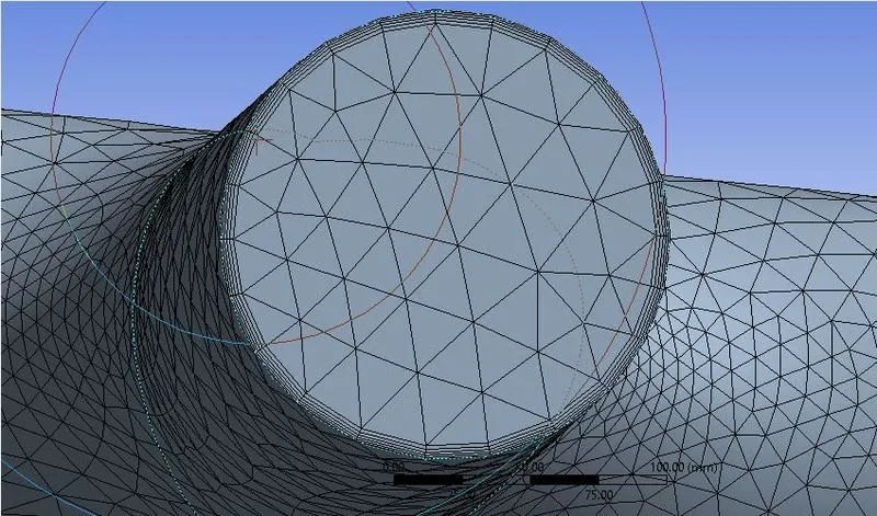
Also, we can see here number of element here

so i think there were something left for improvement and i am going to 'geometry' and show the body so after the analysis i can see that i need to add some of the cells in the solid components.

so for this i am going to use 'sizing'

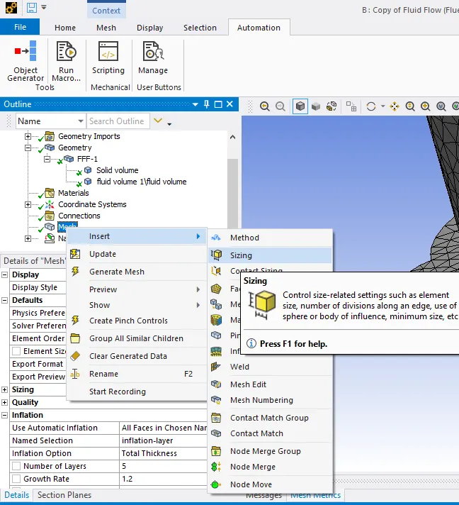
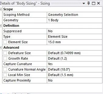
here we can see 'sizing' with 155mm element size

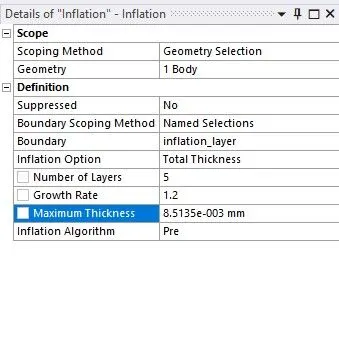
Find the value of y+ in order to provide the value of wall-spacing from the google i.e 0.008513

Results of Case 2:

Mesh size : 150 mm

Body sizing: 15 mm

Solver: k-epsilon

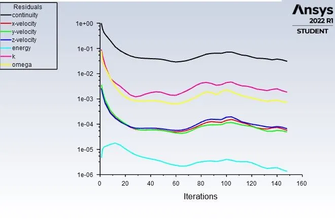
Residuals :

So now move to 'setup' part and run the simulation of 150 iterations.

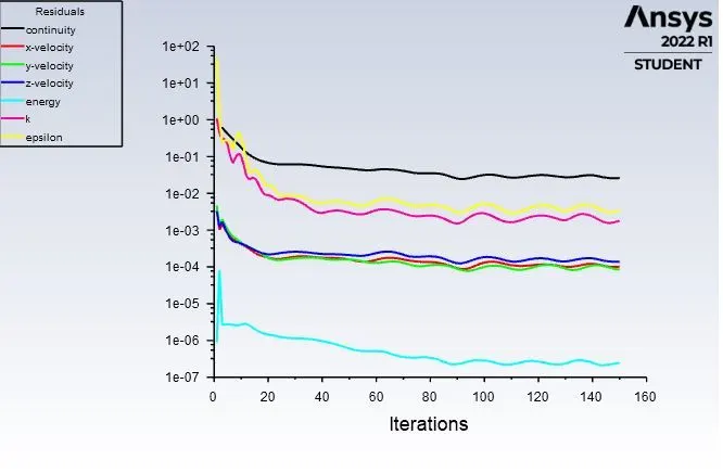
Now move to postsprocessing to see is there any improvements to our heat transfer coefficient.

Velocity Streamline :

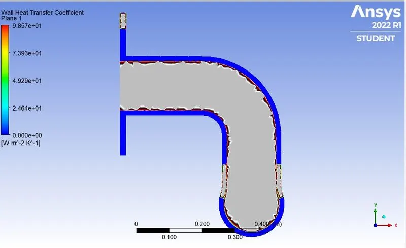
Wall Heat transfer coefficient plot :

Velocity Plot :

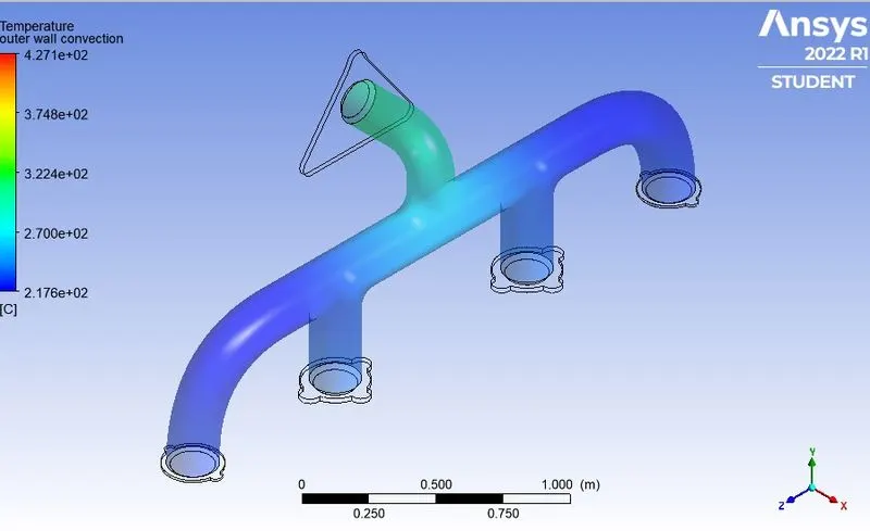
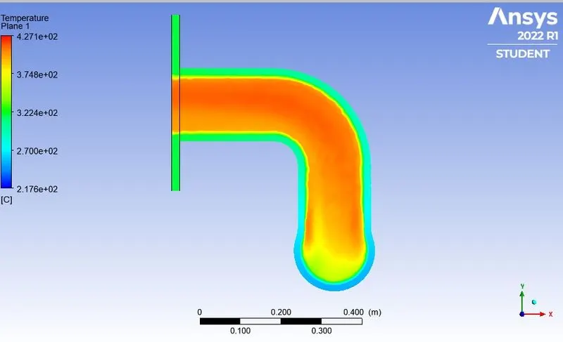
Temperature Plot :

Case 3 :

Mesh Size : 100mm

Body sizing : 20mm

Solver: k-Omega

Residuals

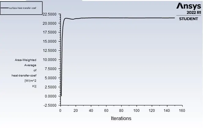
Surface Heat transfer coefficient

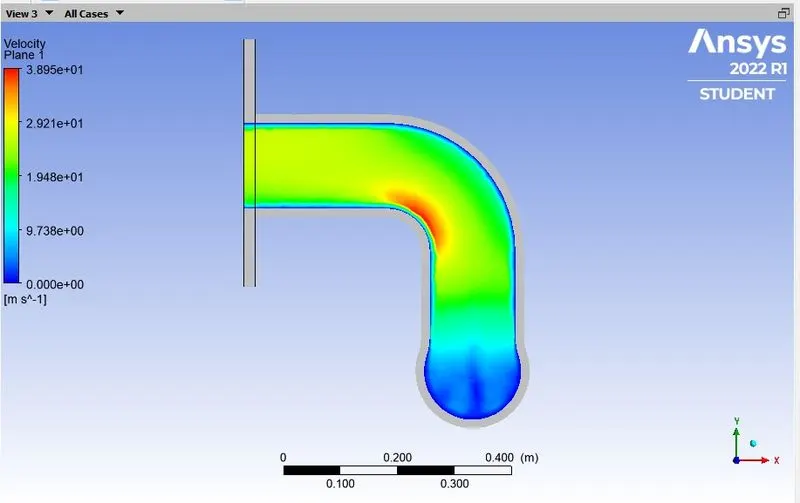
Velocity contour

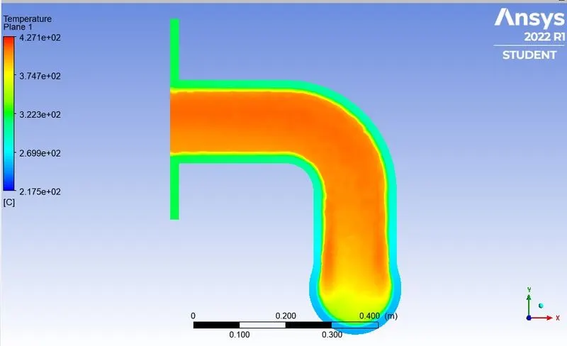
Temperature contour

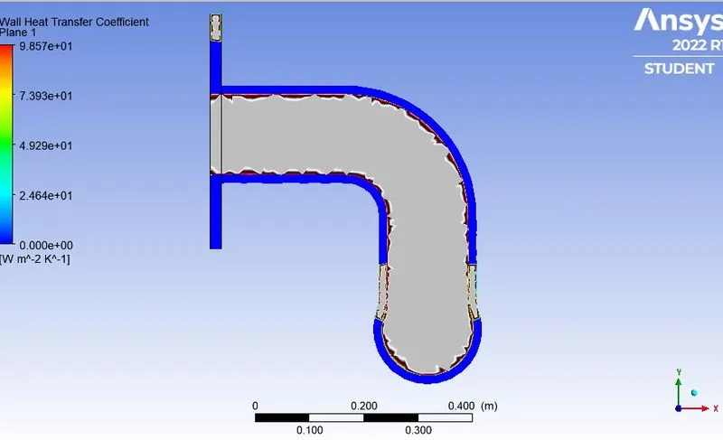
Wall Heat transfer coefficient

Results Discussion: wall heat transfer coefficient and maximumm temperature values are follows

Sr. No.	Viscous Model	Wall heat transfer coefficient (W/m^2K)	Maximum Temperature (k)
1.	k-Epsilon for Baseline mesh	21.186349	575.58234
2.	k-Epsilon for refined mesh	21.408173	592.26648
3.	k-omega for refined mesh	21.416399	591.58569

• No difference in Temperature contours for all three viscous model is observed.
• Maximum heat transfer coefficient is found at layer adjacent to where maximum velocity found.
• Maximum wall heat transfer is found using k-omega viscous model.
• Maximum temperature seen in the k-epsilon in refined case.

Compare the result with the baseline mesh. The refining mesh model gives the result more accurate and optimum. Adding the inflation layer gives the benifits as we can see in the above diagrams. The bending of outlet area produced more Temperature and wall heat transfer coefficient because of high velocity at that region.

HTC VERIFICATION :

Nusselt's number is given by :-

Nu = h. L/K

therefore , h = Nu.K/l

where h = heat transfer coefficient

Nu = Nusselt's number

K = Thermal conductivity coefficient

L - characteristic Length

we know that the Nusselt's number is a function of Reynold's number, which in turn is a function of flow velocity

Therefore, HTC is directly proportional to flow velocity.

Analytical Find the value of Surface-heat-transfer coefficient :

We Know that for Circular tube ,

`Nu = 0.023 Re^0.8 Pr^0.4`

and `Re = {rhovd}/mu`

we know that , ``rho` = 1.125 {kg}/m^3`

``v` = 5 m/s`

d = 0.17 (find this from Area value from 'Geometry')

so, Re = 60457.2119

value of Pr = 0.71 ( from google)

so, Nu = 134.0879

also, `Nu = {hL}/K`

`h = 19.08 W/{m^2 K}

We can see from the images that both the HTC and velocity are maximum near the outlet.

Hence, the HTC predictions from the simulations are correct.

Factors affecting the prediction are as follow : -

1. Element size and Quality = The finer the mesh, accurate the results.

2. Inflation Layer = It increases the quality of mesh near the boundary interface and helps to capture smooth plots of different quantities.

3. Mesh at the solid-fluid interface = The mesh at solid-fluid interface must be conformal.