Week 4 - CHT Analysis on Exhaust port

Objectives:

1. Give a brief description of why and where a CHT analysis is used.
2. Maintain the y+ value according to the turbulence model and justify the results.
   
3. Calculate the wall/surface heat transfer coefficient on the internal solid surface & show the velocity & temperature contours in appropriate areas.
4. How would you verify if the HTC predictions from the simulations are right? On what factors does the accuracy of the prediction depend on?

Introduction:-

The Conjugate Heat Transfer analysis type allows for the simulation of heat transfer between a solid and fluid domains by exchanging thermal energy at the interfaces between them.

Typical applications of this analysis type exist as, but are bot limited to, the simulation of heat exchangers, cooling of electronic equipment and general purpose cooling and heating systems.

CHT analysis can be used to generate increased resolution thermal inputs on the stage wetted surface. Whereas the standard approach uses constant heat transfer coefficients, CHT analysis will export individual nodal Heat Transfer coefficients and Wall Adjacent Temperatures

Procedure:-

Setting up Geometry:-

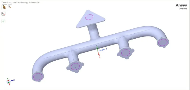
The model can be created in any CAD software and can be imported in Ansys fluent. Here the model is just imported in space claim in stp format.

After importing the model, checking for any repairs to be made before simulation. Checking for extra edges in the model and then extracting the fluid volume.

After the extraction of the fluid volume, the topology will be set to share so that the information will be shared between the different volumes of fluid and solid part of the exhaust port.

Meshing:-

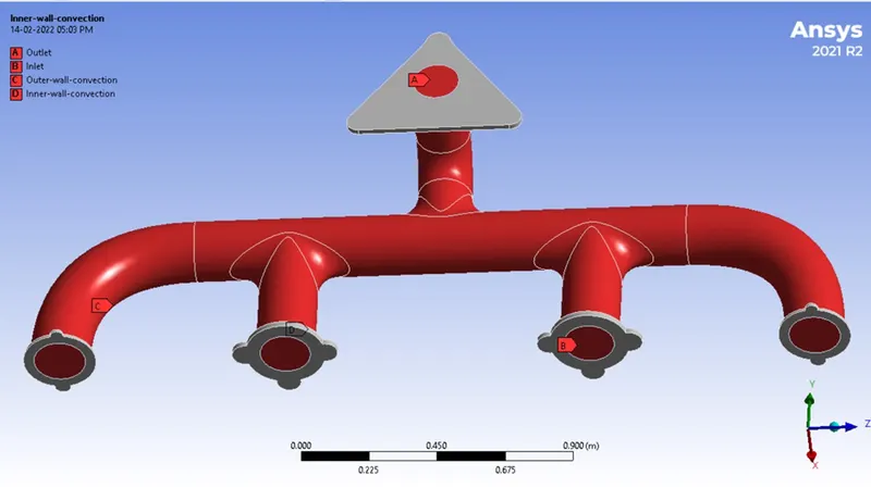
Different named section can be seen below

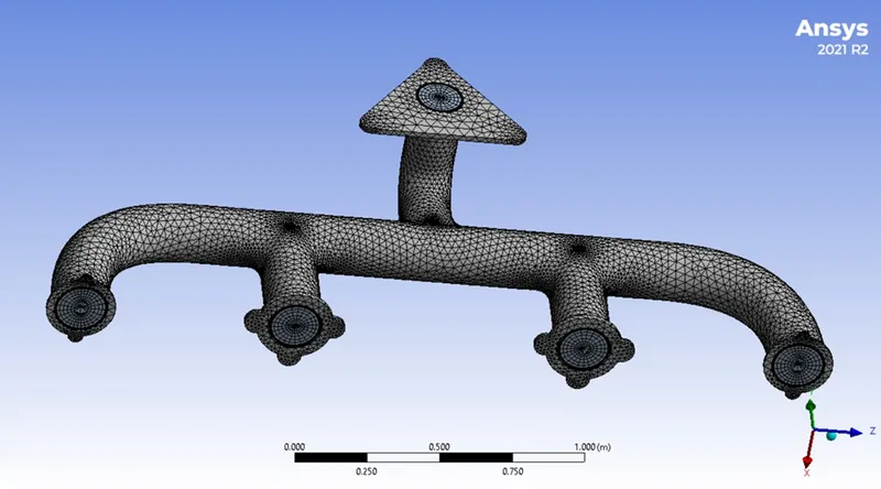
The mesh can be seen below.

The element size for this mesh is 100mm and the total number of elements are 192858.

Determining the Y+ value

Y+ mainly depends on the turbulence model.

For turbulence we need high velocities and close to the wall the velocity will approach to zero. So there has to be a sub layer where the velocity is so small that it becomes laminar and this is the so called viscous sub layer and the question is that whether we can describe this viscous sub layer with the mesh and with the error as the Reynolds average models we assume that we cannot describe this. So the assumption is that our first distance between the wall and our first cell centre is bigger than thus viscous sub layer and e solve it with some kind of empirical equation.

This y+ value just gives us whether we depict this sub layer with our mesh or not and if our mesh is too fine and the y+ value is very low then we don’t have to use the wall functions. The problem is if our mesh is too coarse, because then the assumptions are not correct regarding the height and then the wall functions and then we have to decrease the mesh size. Sometimes due to calculation power and hardware we cannot afford that we just have to know that close to the walls we will always make some kind of errors.

Calculating first cell height

Area – `0.0217 m^2`

Length = 1635 mm

Targeting a Y+ value of 300

Considering the velocity of gas at the exhaust port to be 10 m/s.

Generally, temperatures of 500-700C are produced in the exhaust gases from diesel-cycle engines at 100% load to 200-300C with no load. Exhaust gases normally discharges at a temperature of around 420C.

Considering the temperature of the gas to be 420C i.e 693K

Viscosity of air = `1.81*10^-5` Pa.s

First cell height = 0.0104m

To calculate y+ value

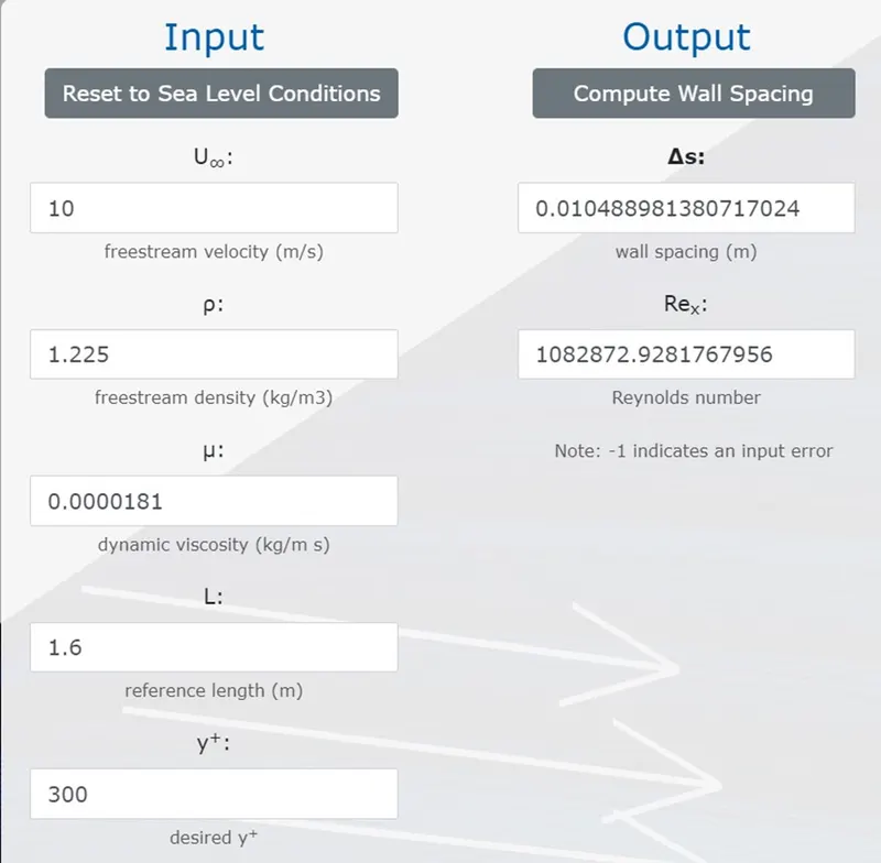
https://www.pointwise.com/yplus/index.html

Setup of Physics:-

Now proceeding towards setting the physics once the mesh is created.

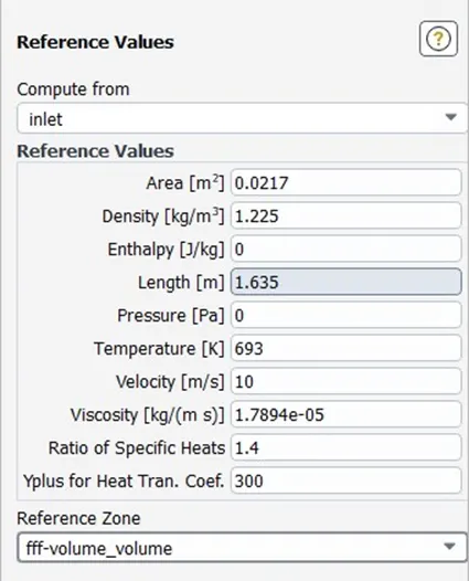
Firstly setting up the reference values as shown below which will be computed from the Inlet

Assigning the fluid to be used as ‘Air’ and the solid part as ‘Aluminium’

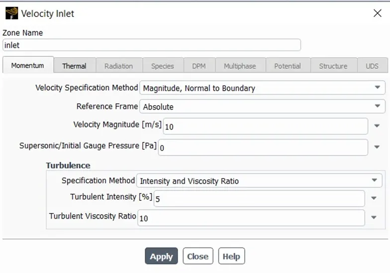
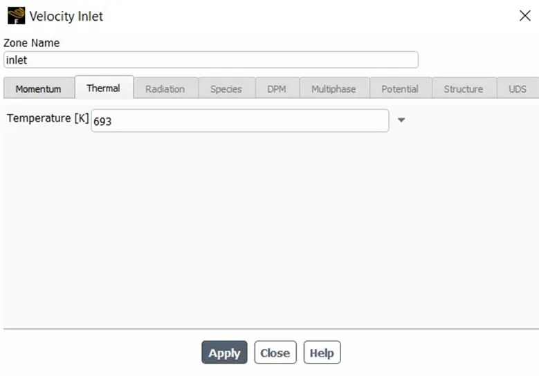
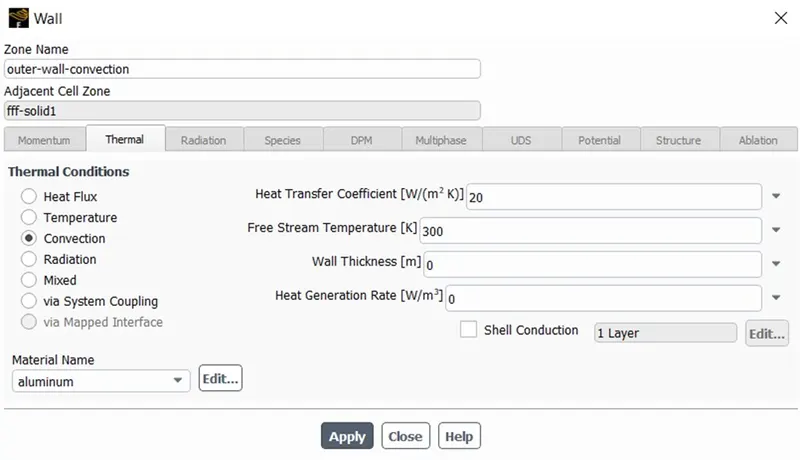
After this setting up the boundary conditions for ‘Inlet’ and ‘Outer wall convection’

Outlet boundary condition will be set as pressure outlet with zero gauge

Inlet boundary condition

Outer-wall boundary condition

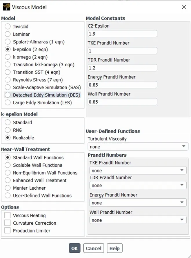
Selecting the Viscous model

Selecting k-epsilon Realizable model with standard wall functions

Starting the simulation with hybrid initialization for 300 iterations.

Post processing

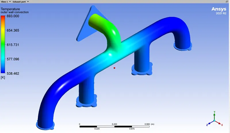
Temperature contour of the Exhaust port

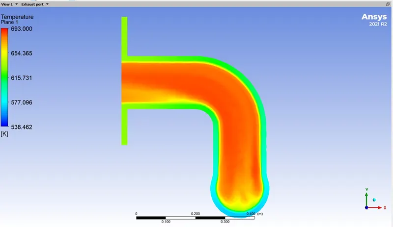
Temperature contour along the plane

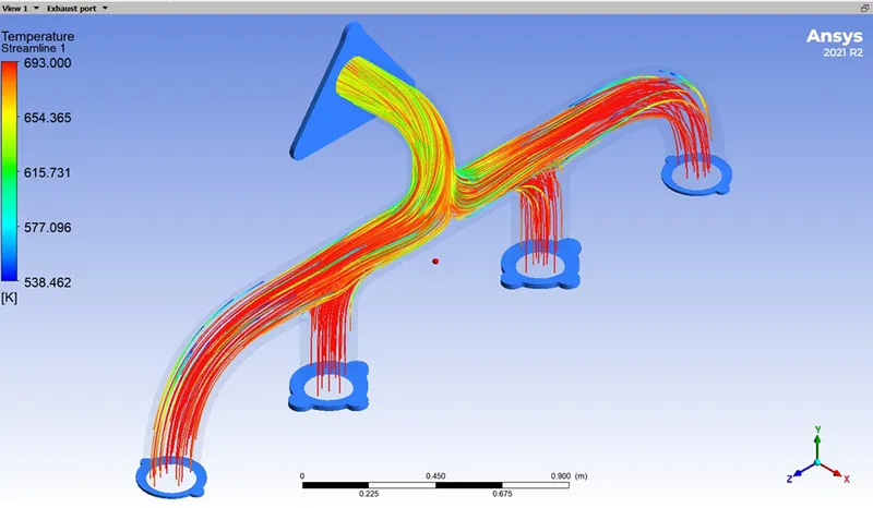
Temperature streamline

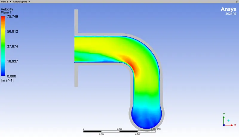
Velocity contour along the plane

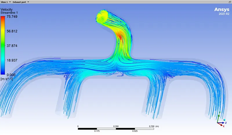
Velocity streamline

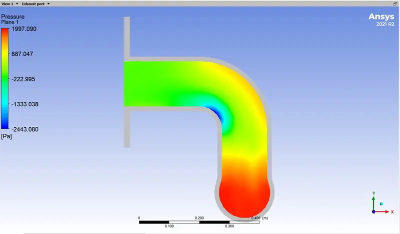
Pressure contour

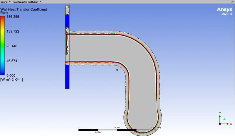
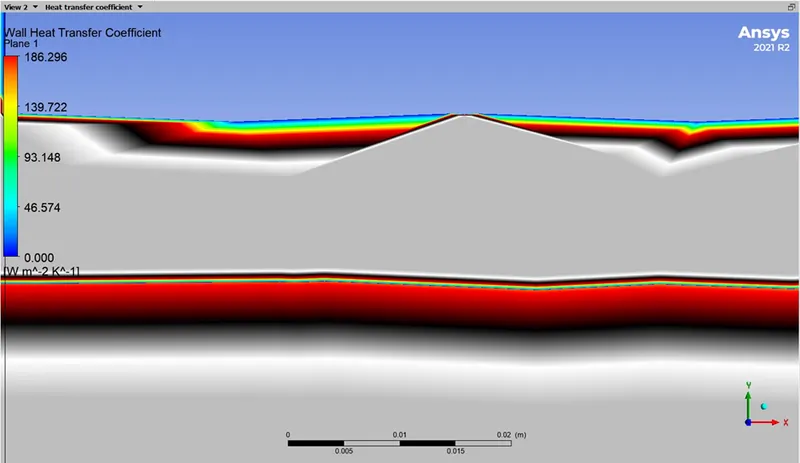
Wall Heat Transfer Coefficient

During the velocity distribution at the mid plane we can see that the velocity at the bend is maximum near the turning.

Also when we see the velocity streamline plot, we observe that the velocity at the inlet is low as compared to the outlet. This is because of mass conservation. The flow rate from all the inlets should match the flow rate at the outlet. This is the reason why the velocity is high at the outlet.

Because of the higher velocity at the outlet, there will be higher Reynold’s number and hence higher will be the Heat transfer coefficient. This means there will be more heat transfer from the fluid to the solid at the location where the velocity is high. This is the reason why the temperature of the solid part is higher at that location.

How would you verify if the HTC predictions from the simulations are right? On what factors does the accuracy of the prediction depend on?

• The accuracy of the result can be validated by comparing with some experimental data
• It can also be validated by theoretically calculating Nusselt number to find Heat transfer coefficient

Calculation of Nusselt Number

It is a dimensionless parameter used in calculations of heat transfer between a moving fluid and a solid body. It is the ratio of heat transferred through convection to heat transfer through conduction.

`Nu = (h*l)/k`

OR

`Nu = 0.023*Re^n*pr^n`

`Re = (rho*U*L)/mu`

Pr = (Momentum diffusivity)/(Thermal diffusivity)

`Pr = (mu*c_p)/K`

Where

`rho`= Density of fluid

`mu` = Dynamic viscosity

K = Thermal conductivity

`c_p` = specific heat

Conclusion:- We can conclude that the model when addition of Inflation layer can trap better wall adjacent values and conditions.

This means that to capture near wall phenomenon, an inflation layer is needed

The finer the mesh, the more accurate the result will be. Good understandings of solvers and models are needed for CHT analysis.