Week 4 - CHT Analysis on Exhaust port
AIM:
The objective of the report is to perform a conjugate heat transfer analysis on the exhaust port and validate the results. The conjugate heat transfer analysis is done in which conduction and convection mode of heat transfer takes place and simulation is performed by using turbulence model in Ansys fluent.
THEORY:
The Exhaust manifold is an important component that affects the performance of I.C engines. Since, after exhaust stroke in I.C engines, the hot exhaust gases along with the sound waves enter the exhaust manifold, the manifold is subjected to high temperature and pressure conditions. The exhaust manifold is attached to the engine cylinder head and has ports that collect exhaust gases from each individual engine cylinder. Since the exhaust manifold is subjected to fast and high-temperature fluctuations, it is generally made up of gray cast iron.
Cracks or leaks in the exhaust manifold leads to decrease in power, acceleration and fuel efficiency of engine.
PROCEDURE:
Cad Model - The Exhaust manifold consists of 4 inlet ports and one outlet port.
Exhaust manifold material - Aluminium
Working fluid - Air
Turbulence model - K Epsilon model
To perform simulation in Ansys fluent, certain steps has to be followed.
Step 1 - Geometry
Import the exhaust manifold cad model in Ansys space claim.
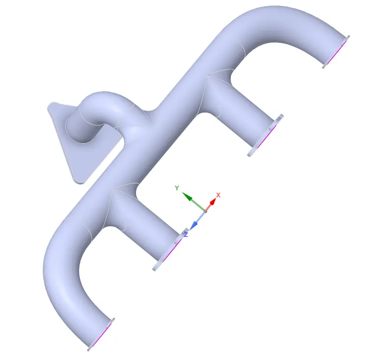
Delete the duplicate edges by REPAIR -> EXTRA EDGES.
In CHT analysis, since the heat is transferred from fluid to solid, the fluid volume should be extracted so that mesh is generated in both sloid and fluid volumes. Extract the fluid volume by PREPARE -> VOLUME EXTRACT.
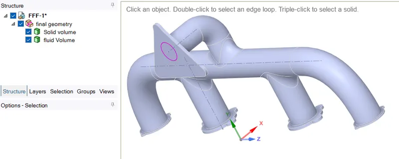
To share thermal information from fluid to solid, it is important to generate the conformal mesh. The mesh at the fluid-solid interface should have proper node connectivity so that a proper flow of information takes place from fluid to solid. To create a conformal mesh, activate share topology. This can be done FFF1 -> ANALYSIS -> SHARE TOPOLOGY -> SHARE.
To share information and to create an interface accurately, go to WORKBENCH -> SHARE.
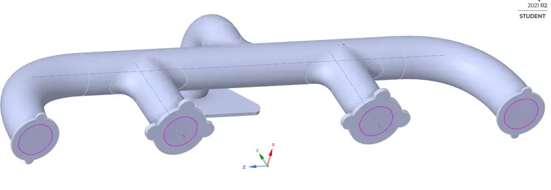
The pink color indicates the interface is generated b/w fluid and solid volumes and proper flow of information takes place.
Step 2 - Mesh
Note - Before generating the mesh, create named selection.
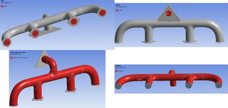
First, generate a mesh of element size - 150mm throughout the domain.
Generate finer mesh in the solid volume of element size 16mm by Inserting body sizing in the solid volume.
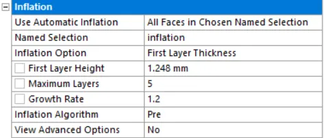
To capture wall effects accurately at the interface, generate inflation layers. The thickness of the inflation layer depends on the turbulence model.
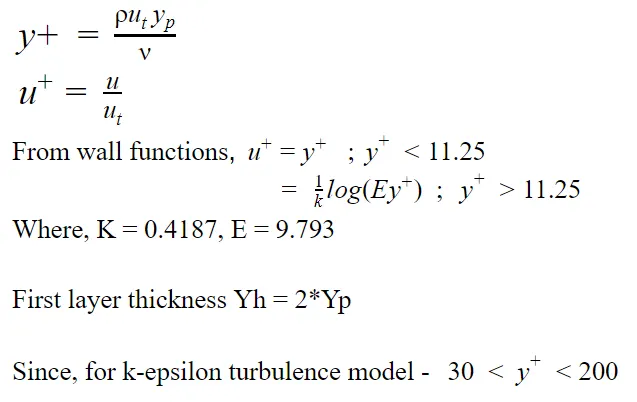
In this report, the k-epsilon turbulence model is considered for analysis, consider y+ as 30.
From the above formulae, we get First layer thickness(Yh) = 1.248 mm. Consider total 5 inflation layers.
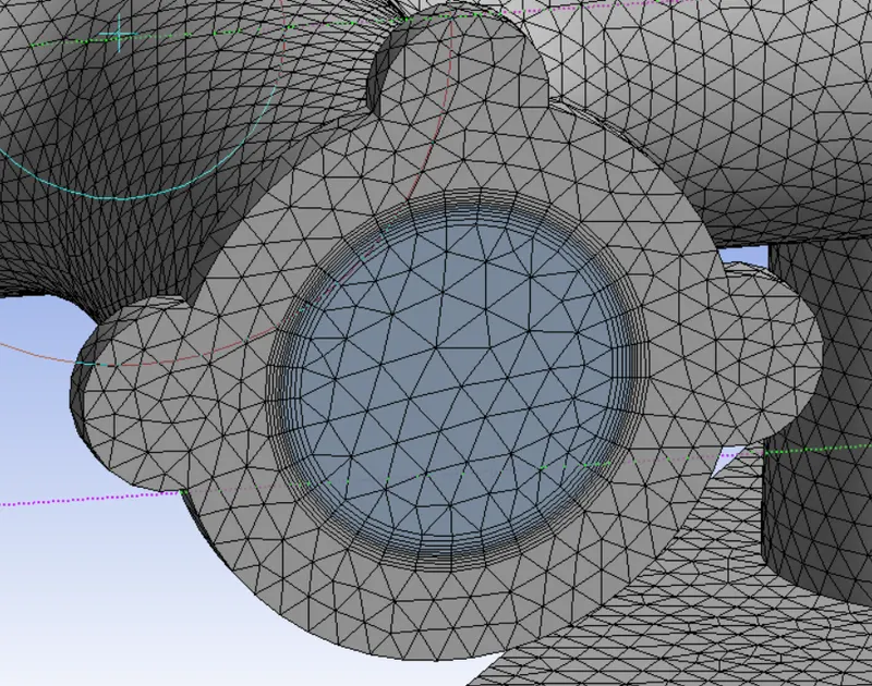
The following fig shows the final generated mesh
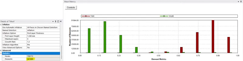
The following fig shows the element quality. The minimum element quality is of 5.34% and the total no.of elements generated are 4,41,688.
Step 3 - Setup
The solver is pressure-based and steady-state analysis is done.
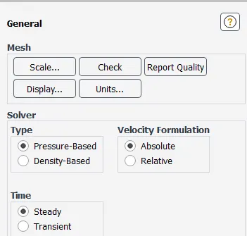
In CHT analysis, Navier stokes energy equation has to be solved. so, check the energy option.

K-Epsilon turbulence model is used.
Material Type - Fluid - Air
Solid - Aluminium
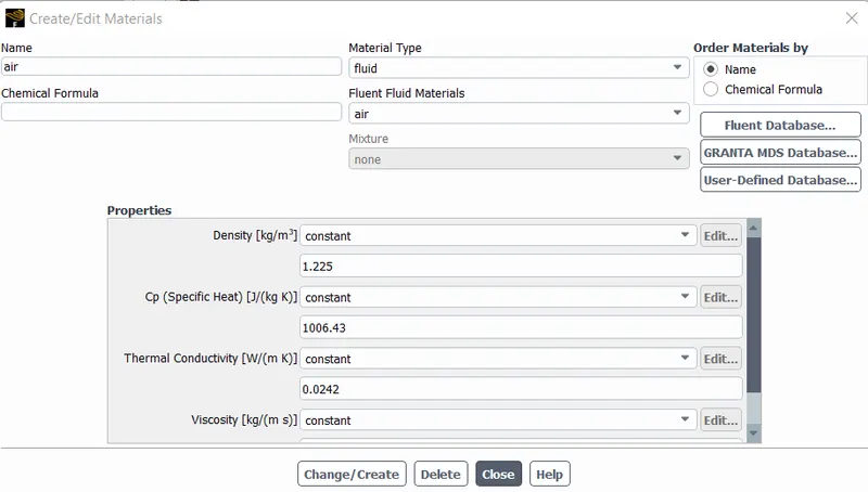
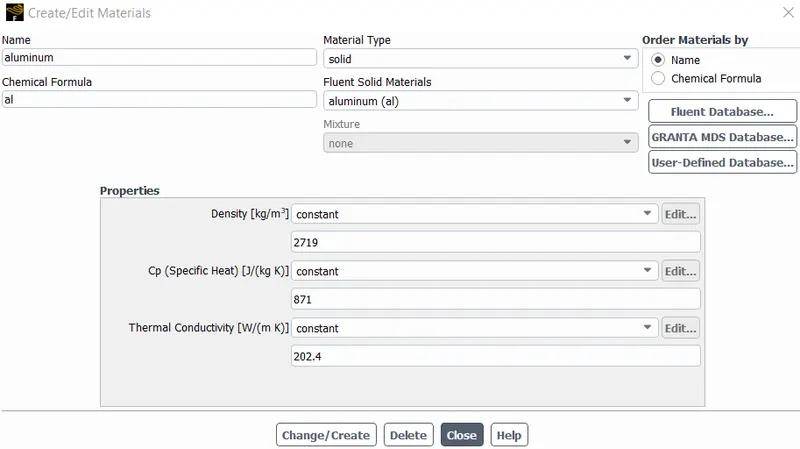
Boundary Conditions -
1) Inlet - Type: Velocity inlet
V = 5m/s, T = 700K
2) Outlet - Type: Pressure outlet
Pgauge = 0 Pa
3) Outer-Walls-Convection - Type: Walls
h = 20 W/m2-K
4) Wall-final_geometry-solid_volume - Type: Walls
Adiabatic boundary conditions
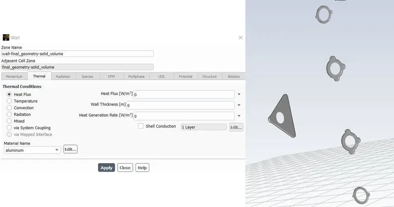
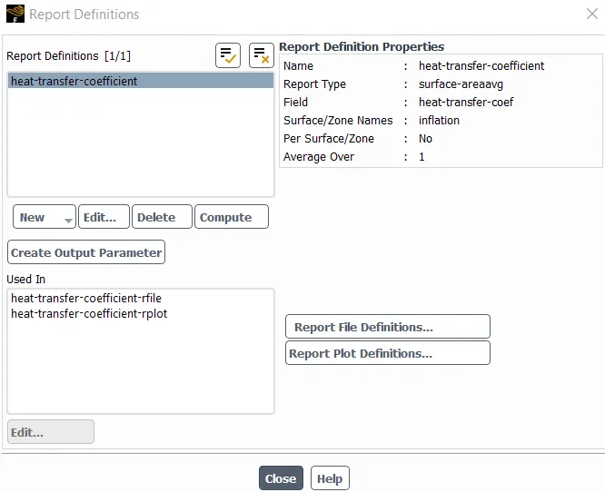
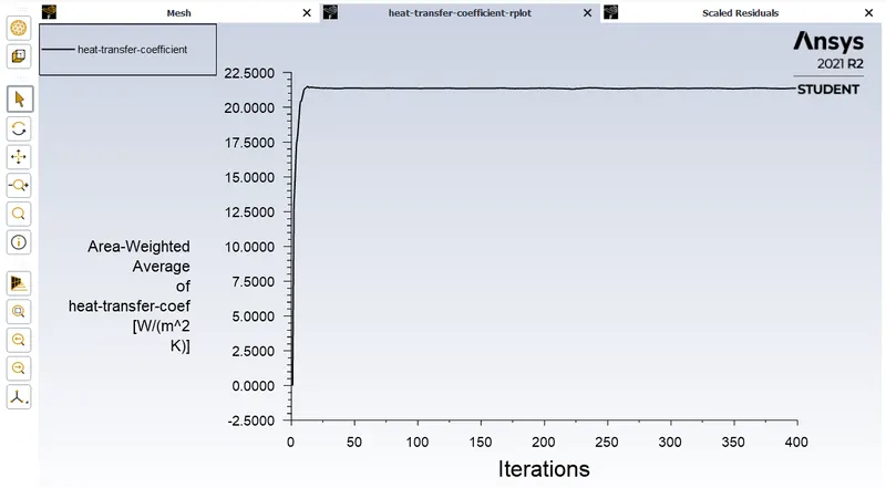
Report - Heat transfer coefficient is computed by using surface average method.
Initialize the model by using Hybrid method.
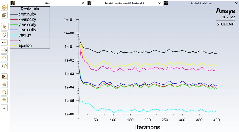
Simulation is carried out for a total of 400 iterations.
Step 4 - Results
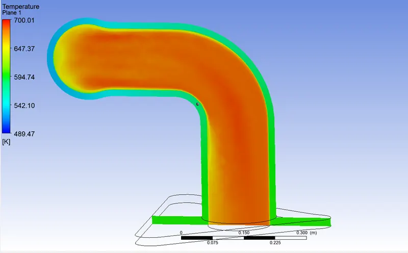
Temperature contour plot of the working fluid on the section of the exhaust port
Velocity vector
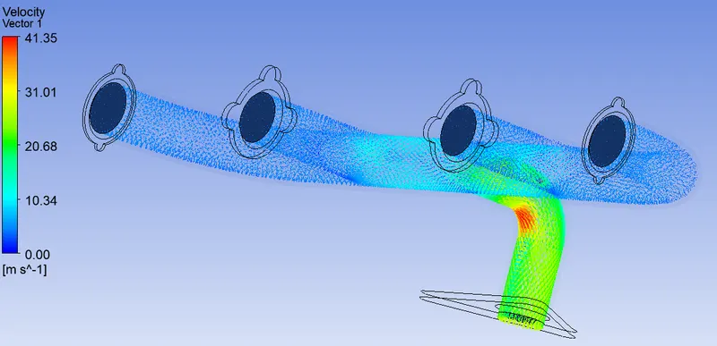
From the fig, it is observed that maximum velocity occurs at the exhaust port section is of magnitude 41.35 m/s. Since, mass is conserved in the entire domain, the maximum velocity occurs at the exhaust port.
Temperature contours on the exterior walls of exhaust manifold
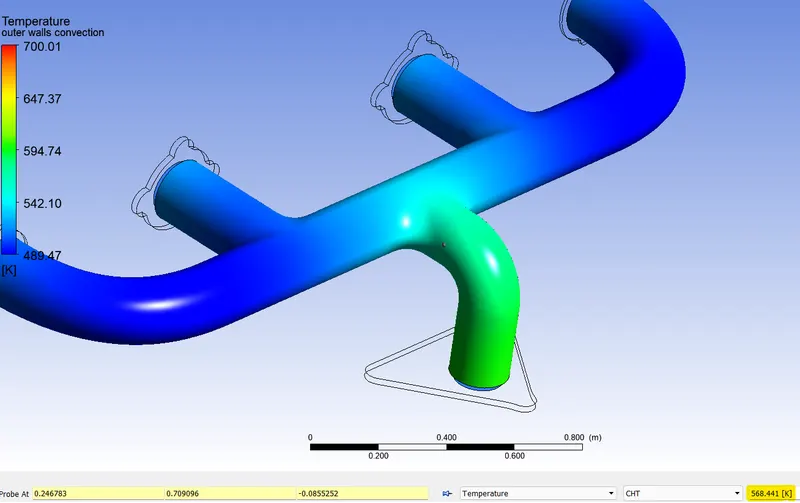
From the fig, it is observed that in the entire domain, compared to the solid surface temperature at the 4 inlet ports, the temperature is maximum at the exhaust port of magnitude 568.44 K. Since, surface heat transfer coefficient depends on the velocity of the working fluid, the heat transfer coefficient is maximum at the exhaust port section, due to which maximum heat transfer takes place from fluid to exhaust manifold at the exhaust port.
The heat transfer coefficient at the interface is computed by using area-weighted average method of magnitude 21.36 W/m2K.
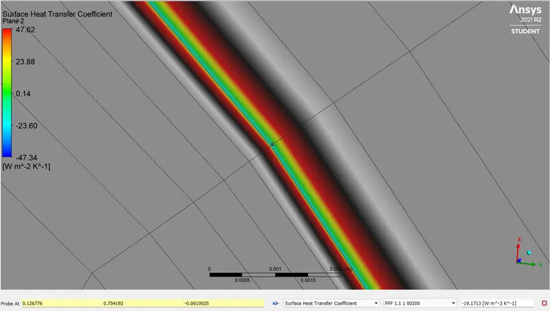
Contours of surface heat transfer coefficient at the fluid-solid interface.
Analytical solution -
The local heat transfer coefficient is analytically calculated by using Dittus - Boelter equation.
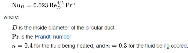
In this model, since working fluid is being cooled in the exhaust manifold, n is taken as 0.3
The characteristic length for the exhaust port is 150mm(Diameter)
Properties of working fluid(air) -
Density = 1.225 kg/m3, Thermal conductivity = 0.0242 W/m-K, Dynamic viscosit = 1.789e-5 Pa-s, Specific heat at constant pressure = 1006.43 J/Kg-K
From the above equation, we get
(hD/k) = 0.023*(V*D/ν)^0.8*(ν/α)^0.3
h = 19.92 W/m2-k
| S.NO | Variable | Analytical solution | Numerical solution |
| 1 | Heat transfer coefficient | 19.92 W/m2-K | 21.36 W/m2-K |
Since, Dittus - Boelter equation is less accurate, the obtained analytical solution is of 7% error.
CONCLUSION:
From the results, it is concluded that since continuity equation is valid throughout the domain, the velocity is maximum at the exhaust port due to which the local heat transfer coefficient is maximum at the exhaust port. Since local heat transfer coefficent value is maximum at the exhaust port, maximum heat is convected from fluid to the solid which makes exterior surface hotter. The heat transfer coefficient at the fluid-solid interface obtained from weigthed average method is of magnitude 21.36 W/m2-K.
The k-omega SST model captures wall effects accurately compared to k-epsilon model. Since in k-omega SST model, y+ < 5 which generates total cell count greater than 6 lakhs which is not possible to perform simulation in Ansys student version. So, the simulation is performed using k-epsilon model.
References -
[1]Wikipedia-https://en.wikipedia.org/wiki/Nusselt_number#:~:text=7%20External%20links-,Definition,flow%20in%20the%20simple%20case.
[2] https://www.ijeat.org/wp-content/uploads/papers/v6i5/E5007066517.pdf