Week 4 - CHT Analysis on Exhaust port

A brief about CHT analysis:

Where CHT analysis is used ?

Conjugate heat transfer is the phenomenon of simulating heat trasfer in both the fluid flow and fluid to solid heat trasfer. I simulteneously solves all relevent flow process equations.

Efficiently combining heat transfer in fluids and solids is the key to designing effective coolers, heaters, heat exchnagers.

Heat transfer in fluids and solids can also be combined to minimize heat losses in various devices. As most gases have small thermal conductivites, they can be used as themal insulators if they are not in motion.

In heat engine parts such as, in exhaust port, cylinder or wherever heat transfer occurs . This calculation helps in design and slecetion of material properties based onnoutput of the simulation.

Effective cooling strategies are critical for various components for emobility systems. Electric motors have high power density and thus generate a significant amount of heat. If motor is not properly cooled, high temperatures in the motor can cause the demagnetization of permemnant magnet and breakdown of winding insulation.

Resolving the spacially varying surface temperature distribution in pumps and compressors improves the accuracy of the simulation and provides useful temperature data.

Simluation procedure:

Step 1 Loading the geometry into SpaceClaim

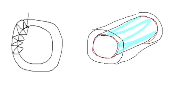
We load geometry into SpaceClaim. Then we use sharePrep option from workbench. When we use this , mesh boundary of two bodys in contact (solid and fluid) they are perfectly interfacing their edges with each other. So, it creates the conformal mesh , there will not be any interference between meshing of solid and fluid meaning zero distance between two meshes.

When we hit Share , this red coloured boundary is shown where the faces of meshing boundary of two bodies are interfacing with each other.

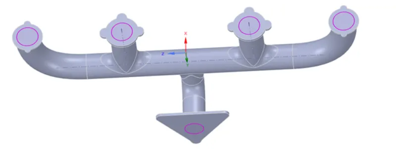
And surface boundary of two faces become pink means share option is enabled and the boundary is shared.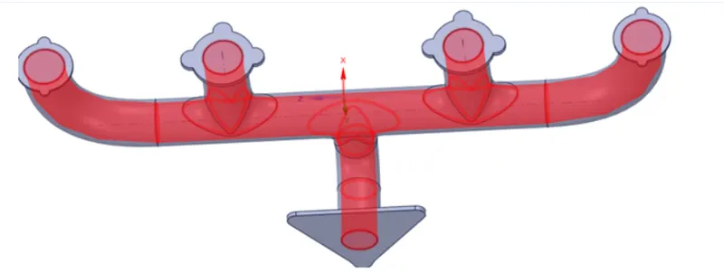

Step 2: Meshing

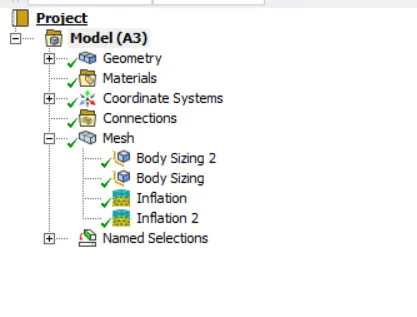
In the meshing, we first create baseline meshing. Then as we observe thats not finer mesh we require, we insert sizing and inflation as below,

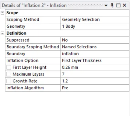
Here, concept of Yplus is very important to understand. So we want to catch the physics near the wall. We want to model total turbulence layer hence let us assume first node to be in viscous sublayer. As Yplus of 1 to 5 gives the node in viscous sub layer, we assume Yplus 5 in this case, and be below calculation let us calculate the frst layer thickness,

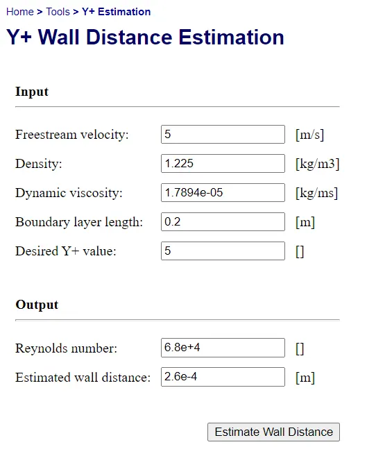
So first layer thickness comes as 0.26 mm.

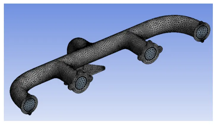
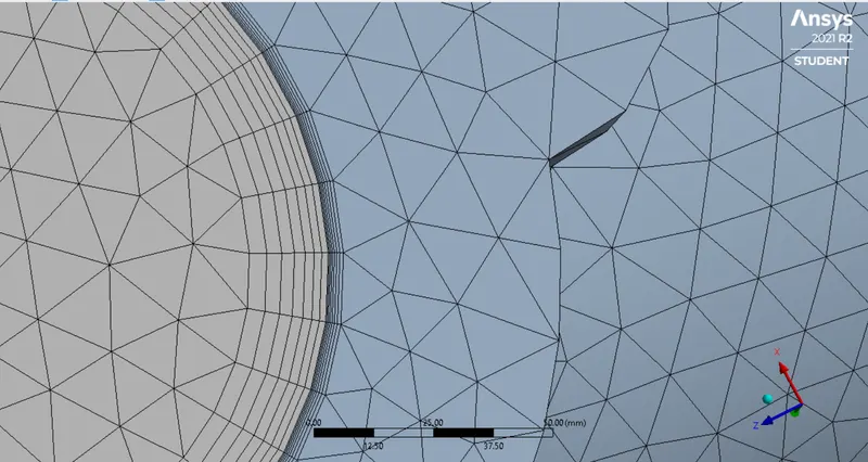
Mesh Quality

a) Orthogonal

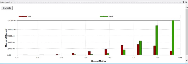
b) Skewness

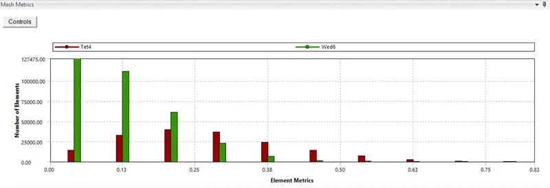
Step 3: Set up

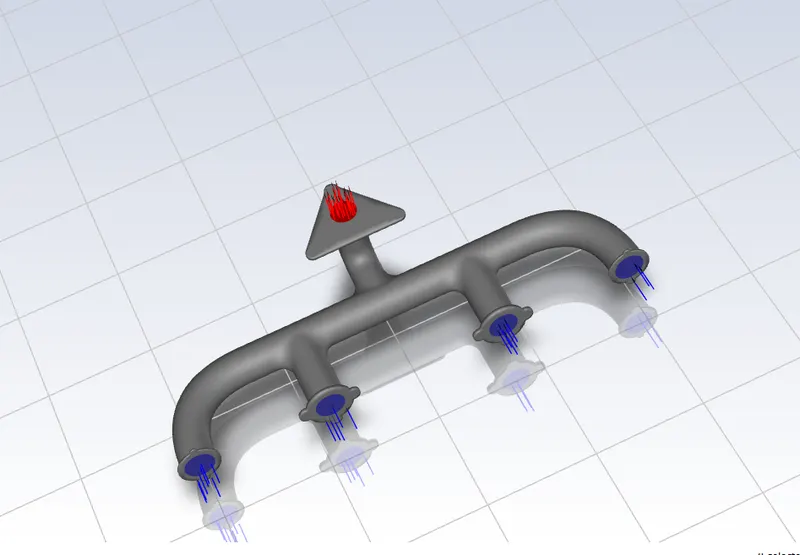
In set up, we provide the information or input for the simulation for simulation. So , when we open setup, we see blue arrows for inlets and red for outlet.

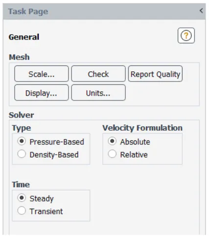
General settings

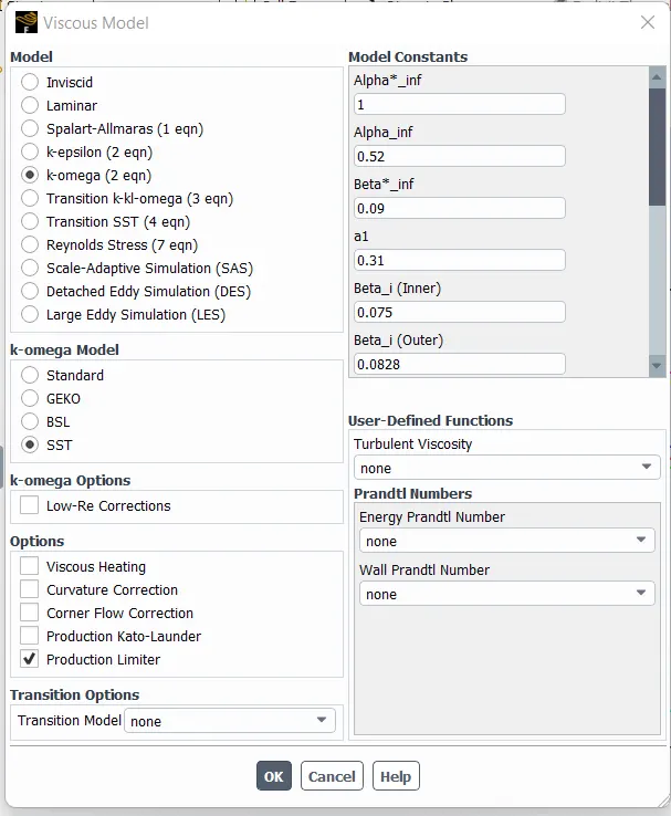
We are going to set viscous model tp k-w as we want to capture near wall effects.

Boundary conditions are as below,

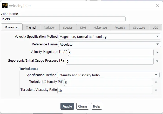
inlet as velocity inlet with v =5 m/s and temperature as 700K under Themral tab.

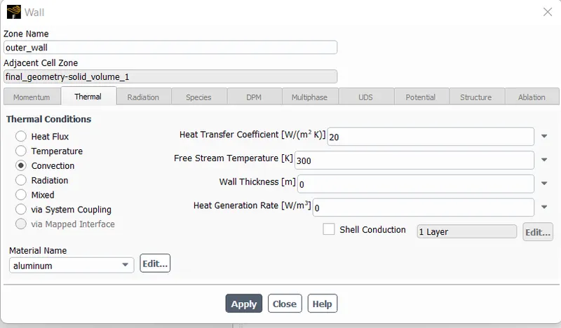
for wall, heat transfer mode is going to be convection and coefficint we are considering 20 W/m2K. Generally finding h is not so easy task, it depend supon the experimental conditions. Or we have to take another CFD simulation.

Next is materials , we have used air for fluid material and aluminium for solid which were default values.

After set up, we create the contour of velocity and temperature.

Results:

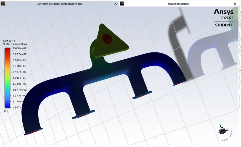
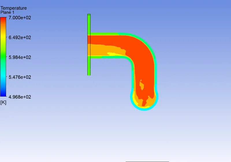
a) Temperature contour :

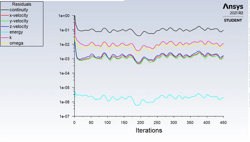
b) Scaled residuals

c) Velocity contour

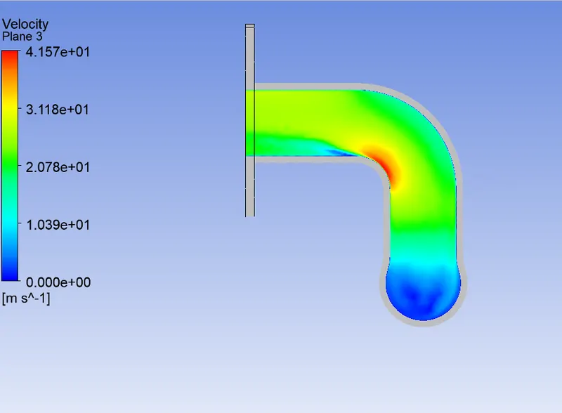
We see that there is much more velocity accounted at red region in contour. Hence, there will be more Reynold's number, more heat transfer coefficient also.

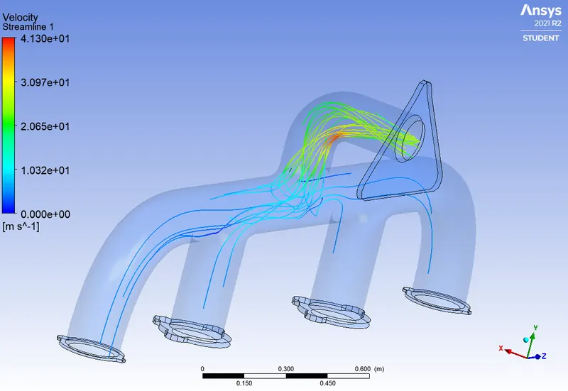
Velocity streamlines

c) Wall heat transfer coefficient

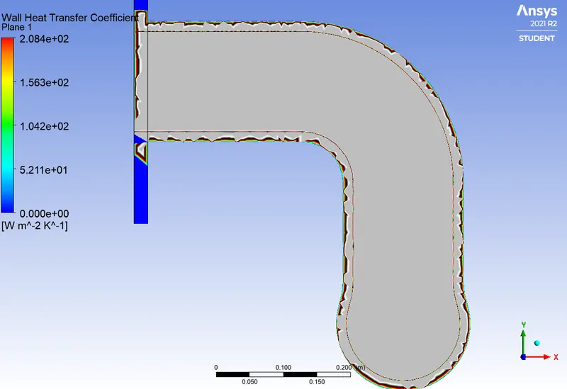
CFD POST

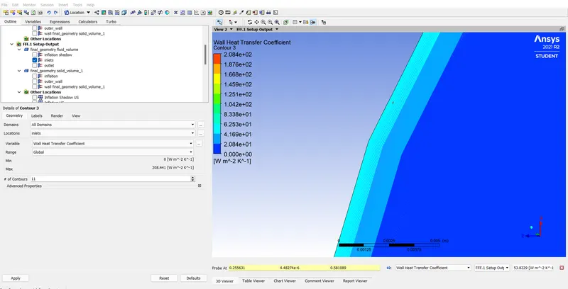
h value at inlet

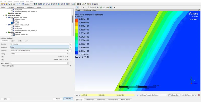
h value at outlet

Case 2

Now, we refine the mesh by reducing the Y+ value of wall.

Let us change from 5 to1.

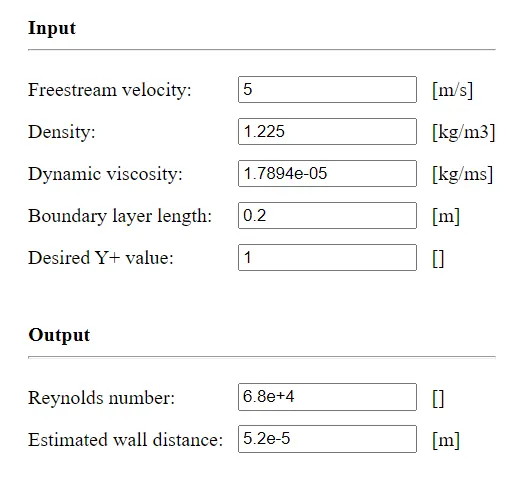
In this case, set up and geometry remains the same while the meshing and solution changes.

Let us discuss about meshing.

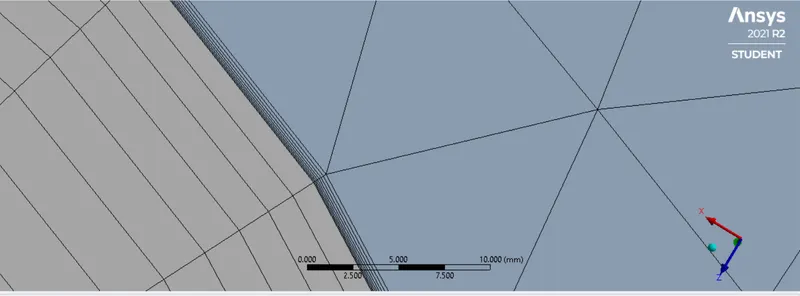
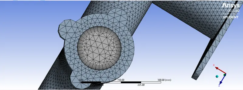
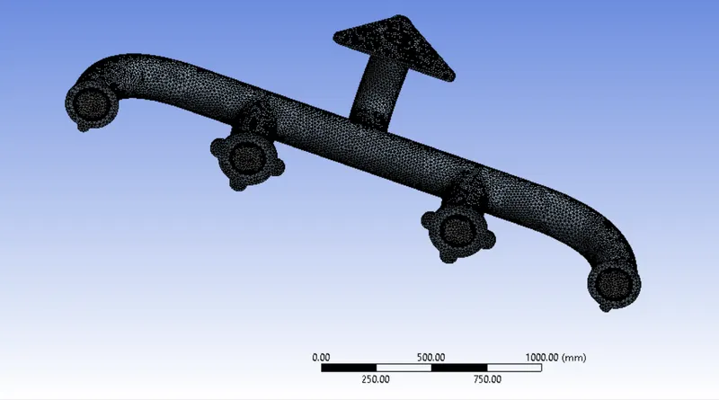
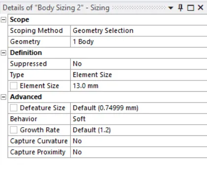
Mesh parameters are as below,

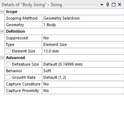
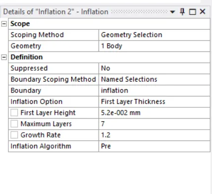
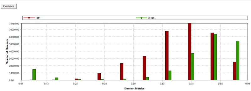
Mesh Quality:

1) Orthogonal Mesh Quality

2) Skewness Quality

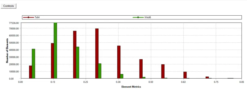
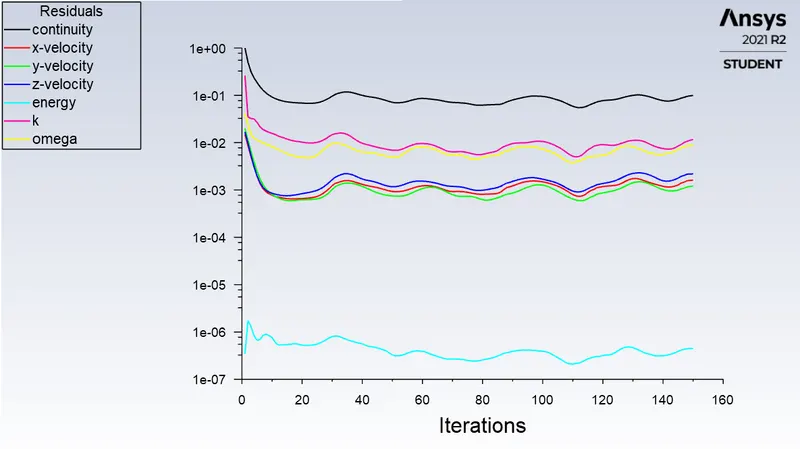
So, we update mesh after this and open set up .Then we initialise the solution and calculate for 200 iterations.

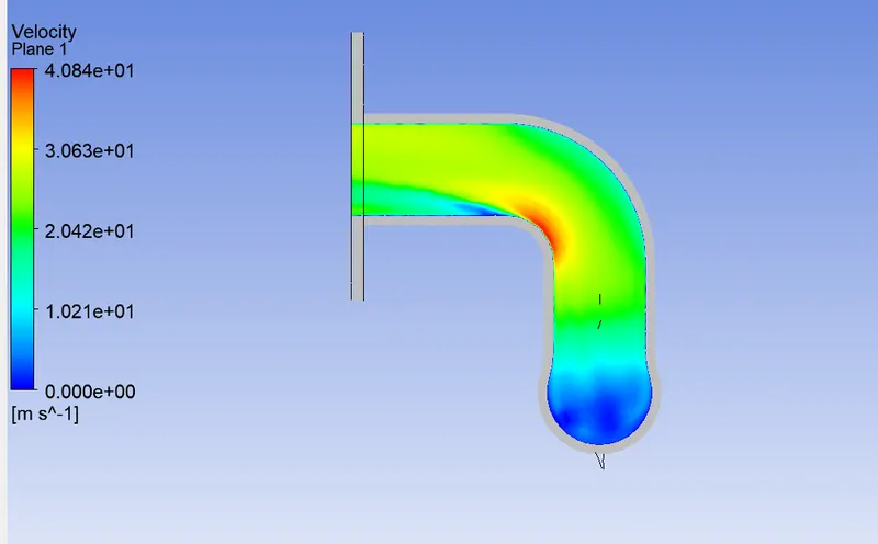
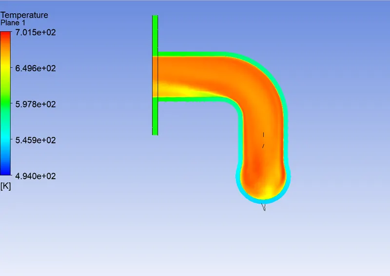
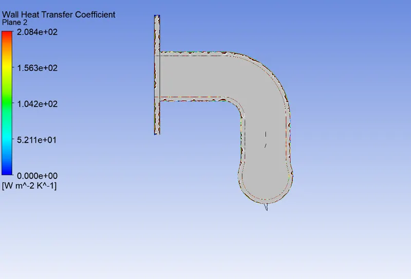
We get below results.

a) Scaled residuals

b) Velocity contour

c) Temperature contour

d) Wall heat transfer coefficient

Validation of CFD simulation

Let us consider one case out of the above two for validation purpose.

Case 2

Here we have considere yplus of 1 and below are the values for analytical calculation of h at inlet and outlet.

Heat transfer coefficient at inlet

Nu = hL/k

h = k. Nu/ L

where k is thermal conductivity of fluid = 0.025 W/m-K

L, is Hydraulic diameter

Nu is Nusselt number

Nu = 0.023* Re^0.8*Pr^0.3

Re is Reynold's no. and Pr is Prandtl no.

Re = Ro*v*D/Mu

= 1.225*5*0.2/ 1.789e-5

= 6.8e+4

Pr = Mu*Cp/k = 1.789e-5 * 1075/0.025 = 0.7949

Nu = 157.699

h = 19.71 W/m^2-K

So, at the inlet, velocity is much less hence causes less heat transfer.

Heat transfer coefficient at outlet

Nu = hL/k

h = k. Nu/ L

where k is thermal conductivity of fluid = 0.025 W/m-K

L, is Hydraulic diameter

Nu is Nusselt number

Nu = 0.023* Re^0.8*Pr^0.3

Re is Reynold's no. and Pr is Prandtl no.

A2*v2 = A1*v1

A2 = 4* A1

So, V2 = 4*v1 = 20m/s

Re = Ro*v2*D/Mu

= 1.225*20*0.2/ 1.789e-5

= 2.72e+5

Pr = Mu*Cp/k = 1.789e-5 * 1075/0.025 = 0.7949

Nu = 478.05

h = 59.756 W/m^2-K

So, at the outlet, velocity is high which means a high Reynold's number which leads to a high heat transfer rate , hence high heat transfer coefficients.

Above analytical calculation we did is for simple pipe flow. But we did simulation of exhause pipe which is much complicated geometry and many bends are there in between. So, we can never expect the accurate comparison, but we can defiitely know the range of results.

h values by simulation in CFD post

a) inlet

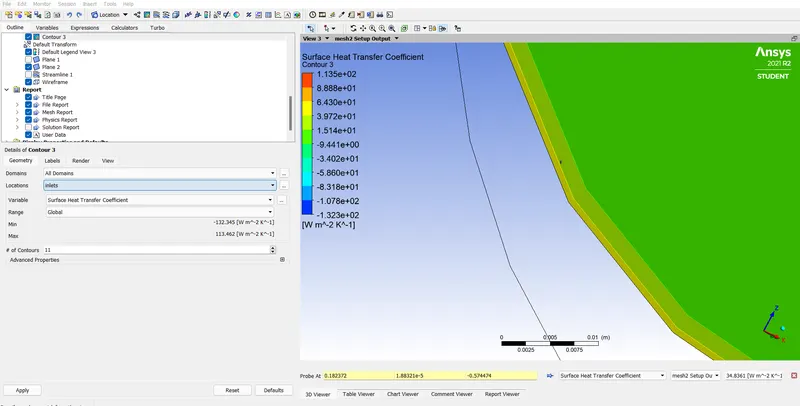
h = 34.8361 W/m^2 K

b) Outlet

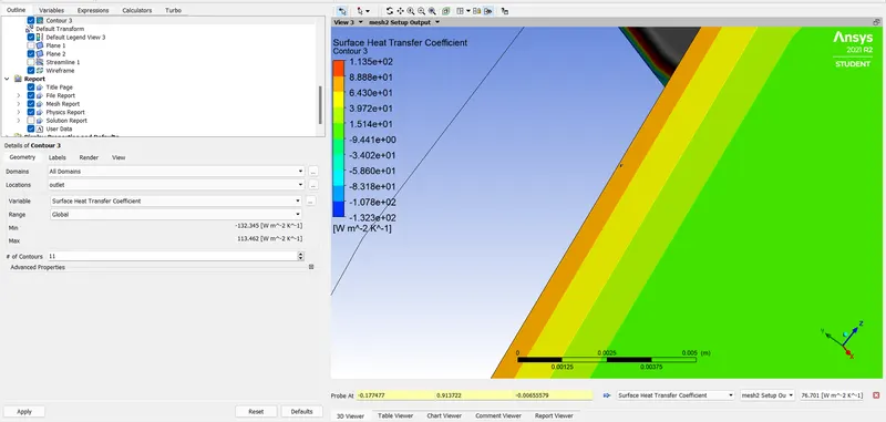
h = 76.701 W/m^2 K

• Validation table

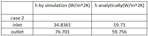
Comparison table for h values from simulation

Conclusion:

• For turbulence models in program, we have to take care of Y+ value and boundary conditions. Meshing also plays important role. Coarse mesh will not give accurate results. So, we have to refine geometry to catch important phenomenon that are happening near wall or some special areas.
• There are few factors which we have to consider which are most significant are turbulent boundary layer, Y+ value. So, when we are using RANS model , in that k-w SST model, we need to stay in Viscous sub layer of turbulent boundary layer, where velocities are assumed to be laminar and viscous stress dominates the wall shear meaning Y+ <5.
• Motivation to use k-w model instead of k-e is to address the shortcomings of k-e model in dealing with near wall treatment. So, k-e works well for those flows where we want to capture only those regions where adverse pressure gradients are not present and those are core turbulent flows. So, omega based models use blending function F1 which is best for core turbulent flow and near wall also.
• In Fluent, reference temperature is important in determining heat transfer coefficient.