Week 4.2: Project - Transient simulation of flow over a throttle body
Introduction:
Defnition of throttle valve
A valve designed to regulate the supply of a fluid (as steam or gas and air) to an engine and are operated by a handwheel, a lever, or automatically by a governor. Especially : the valve in an internal-combustion engine incorporated in and are regulated for controlling the volume of vaporized fuel charge delivered to the cylinders.
A throttle is the mechanism by which fluid flow is managed by obstruction of a throttle.
An engine's power can be increased or decreased by the restriction of inlet gases (by the use of a throttle), but usually decreased. The term throttle has come to refer, informally, to any mechanism by which the power or speed of an engine is regulated, such as a car's accelerator pedal. What is often termed a throttle (in an aviation context) is also called a thrust lever, particularly for jet engine powered aircraft. For a steam locomotive, the valve which controls the steam is known as the regulator.
In an internal combustion engine, the throttle is a means of controlling an engine's power by regulating the amount of fuel or air entering the engine
To regulate the power output from an engine there have to be some restriction of how much fuel - air mixture that reaches the cylinders. One way to do this is to use some kind of valve that restricts the air, fuel is then regulated to get the correct fuel - air mixture.
Objective: To perform a steady state simulation in a an elbow consisting of an throttle body in it in order to analyze the flow parameters and the fluid behaviour in the vicinity of the nozzle inside the throttle body.
The geometry and the Case setup is same as steady state. The only preparation required for transient case is the rotation of throttle valve in the elbow joint. After hiding the elbow geometry we enable only the throttle valve. To rotate the valve we need to find its center of axis and normal of the valve about which we desire rotation.
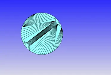
We need to hide the rest of the surfaces except the cylindrical shape shown below and keep these enabled, as the center of the throttle valve is the centre of the rotation. So, we used Measure tool and select the Arc normal and following that we select 3 vertex on the arc of the below shown cylindrical body. This gives the value of arc center and arc normal values which we copy and paste and apply in the Boundary condition of the throttle instead of law of wall as we selected before in case of steady state. More details are provided in Case setup.
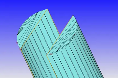

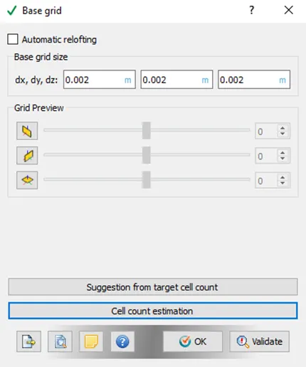
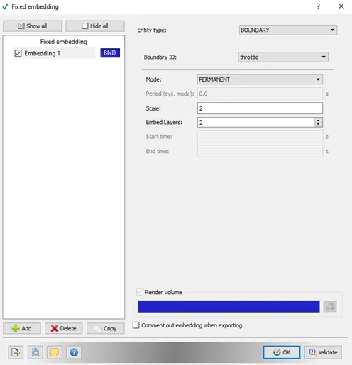
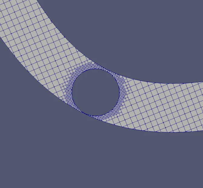
The mesh is kept slightly Coarse than the steady state here just to save computational time. The element size is 0.002 m with fixed embedding of 2 scale and 2 layers as we applied in steady state simulation as well.
Total cell count
The total cell count is actually not constant because of the rotation of the throttle valve for which our mesh is being continiously refined .The cell count is varying exactly on the time of flow we have rotated the valve to a specific angle(25 deg here in the present study) and becomes constant when its not rotating or we can rather say that when it comes back to its original position after one rotation. The maximum flow time is 0.01 s.
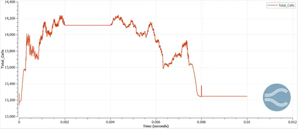
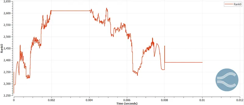
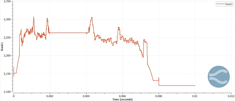
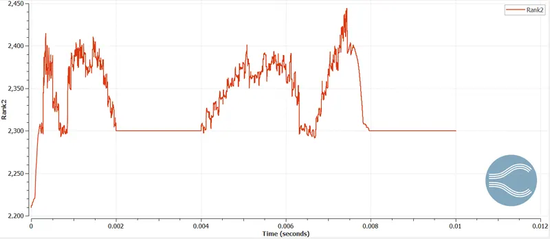
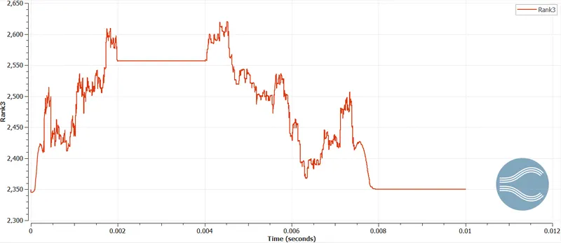
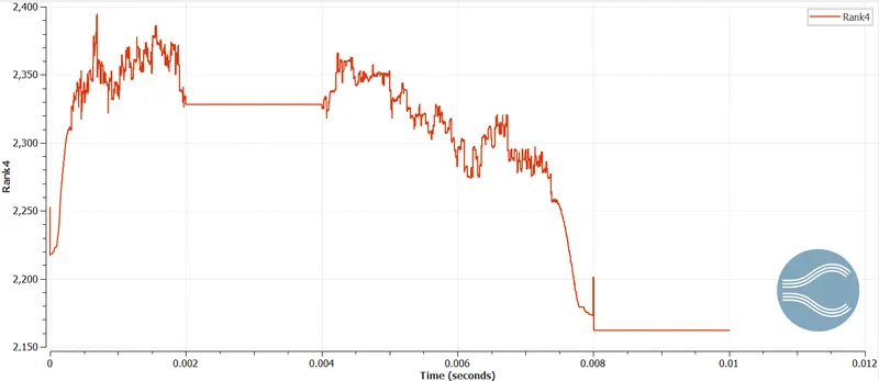
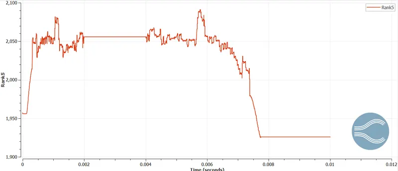
Since we are rotating the valve to 25 degrees from 2 to 4 m/s total cell count has a specified value when throttle valve starts rotating and with the application of fixed embedding, it helps us to provide the desired no of cell counts to capture data throughout rotation process. The total cells keeps on changing with the rotation of the valve.
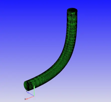
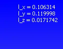
From the dimensions of the elbow we can predict the flow time and end up in deciding the end time which is 0.01 s.
If we assume the total length to be 0.2 m in the xy direction and from the steady state solution it was observed that the avg flow velocity was above 180 and near to 200 m/s at the outlet. For the sake of convenience if we consider 200 m/s as the average flow then the total time for one complete flow will be 0.001 s. So if we want 10 such total flows it will result in 0.01 sec as the end time.
Case Setup( all same except the boundary condition of the throttle valve and the simulation run parameter which is because of transient simulation)
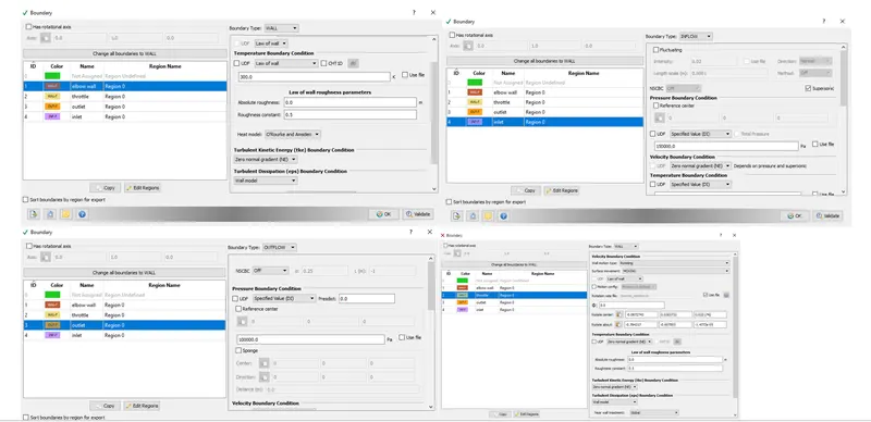
Boundaries were created namely, elbow wall, throttle, inlet and outylet and proper Boundary conditions were assigned to them according to requirement.
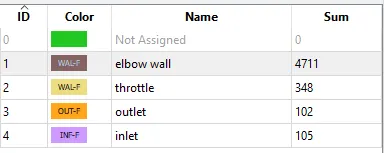
Application: General Flow
Material: Gas simulations and Global Transport propertiers were set as default.
Boundary conditions: Elbow(Boundary Id 1) and throttle were assigned ROTATION boundary type with all the rotation conditions(axis of rotation, rotation centre).Inlet(Boundary id 3) boundary type inflow and pressure =150000 Pa, species inflow O2 and N2. Outflow (Boundary id 4) boundary type outflow and pressure=100000 Pa, Species :- O2 and N2. All boundaries are assigned Region 0.
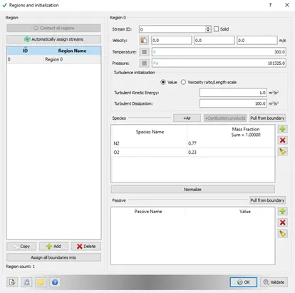
Regions and initialization: Temperature 300 K, and pressure= 101325 Pa, Species Air (O2 and N2).
Physical modeling: Turbulence modelling with RNG
Run Parameter under the Simulation Parameter
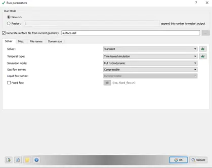
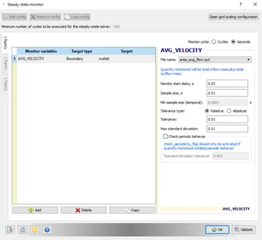
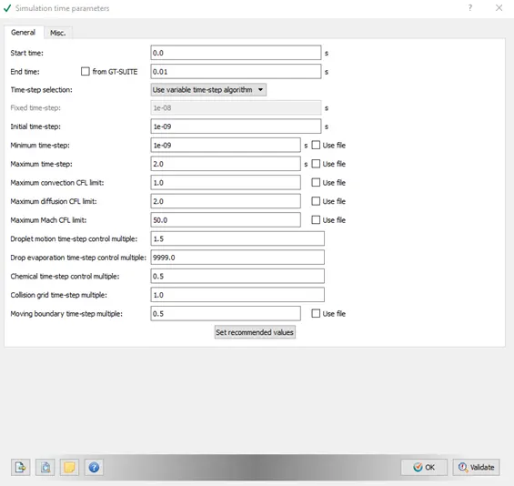
Steady state pressure based solver was chosen under the solver tab, flow mode was set to the Full Hydrodynmic under the simulation mode and Compressible flow was chosen under the Gas flow solver. In the Miscellaneous tab, steady state monitor was checked on and use shared memory was unchecked because sterady state simulation is performed
Base Grid Size
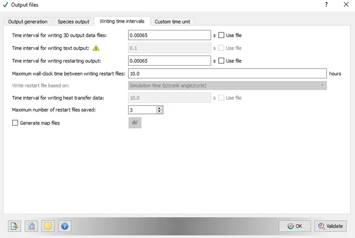
Output files: Total 16 output files were extracted and analyzed in paraview
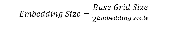
Fixed embedding is applied to refine the grid at specific locations in the domain where a finer resolution is necesasary for the accuracy of the solution. Fixed embedding allows the rest of the grid to remain coarse to minimize simulation time. For each fixed embedding, one must specify an embedding scale that indicates how CONVERGE will refine the grid in that location(here in this case the vicinity of the throttle valve). The embedding embed_scale parameter in embedded.in, which must be a positive integer, scales the base grid sizes according to the formula
Post Processing Results
Velocity and pressure contour:
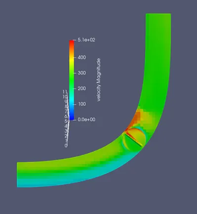
The maximum velocity attained is increased from the steady state, its around 510 m/s for transient case whereas it was around and within 200 m/s for steady state. The physics of the flow and velocity distribution is same ias n the steady state except for the profile of average velocity value itself. The contour is for the last flow time 0.01 second.
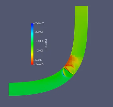
The max pressure set 2,40,000 Pa. The lowest pressure observed decreased that observed from the steady state. The low pressure obtained near the cylinder region of the throttle is due to its shape when the throttle body provides least hindrance to flow where velocity is max.
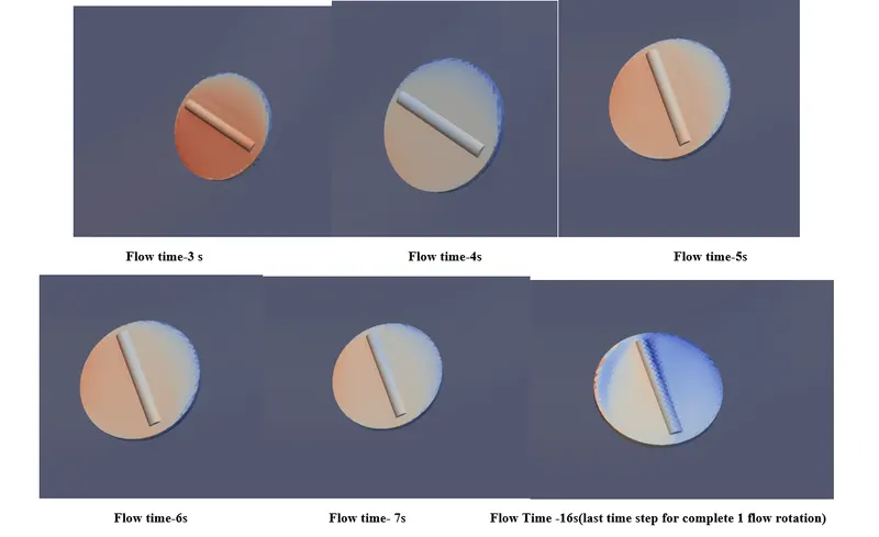
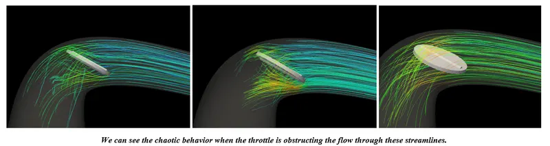
Animations are attached at the end for clearer view.
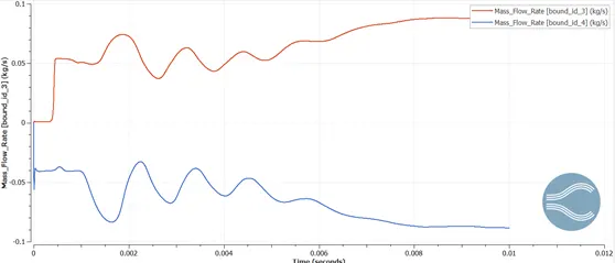
Plot for Mass Flow Rate
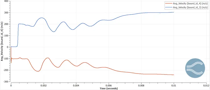
Plot for velocity average at the inlet and outlet
In the initial valve is in opening position which we can easily observe in the below figure that in the start velocity goes smooth after 0.001s velocity is going to decrease at the outlet. At a time 0.002s valve is in 25 degree position means we can say that valve is in closing position, there is decrease in velocity before that . From 0.004s throttle valve is again starting to open, we observe that there is a little increase occuring in velocity. All the increase and decrease in velocity is accompanied by fluctuations and wake regions because of the movement of the throttle. After,008s velocity profile is smooth and becomes steady because at that position throttle vave is again open i.e it reaches back to it’s original position.
Plot for Total Press and Static Pressure at the outlet
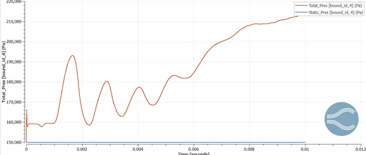
The variation of other plots is pretty much the same as discussed in steady state.
Animations: