Week 4.2: Project - Transient simulation of flow over a throttle body

Aim:

1. Setup and run the simulation.
2. Plot pressure, velocity, mass flow rate, and total cell count and show the velocity and pressure counters.
3. Study the results and analyze the flow happening over and around the body.

Theory:

Throttle body:-

A throttle is a mechanism by which fluid flow is managed by constriction or obstruction. An engine's power can be increased or decreased by the restriction of inlet gases (by the use of a throttle), but usually decreased. The term throttle has come to refer, informally, to any mechanism by which the power or speed of an engine is regulated, such as a car's accelerator pedal. What has often termed a throttle (in an aviation context) is also called a thrust lever, particularly for jet engine-powered aircraft. For a steam locomotive, the valve which controls the steam is known as the regulator.

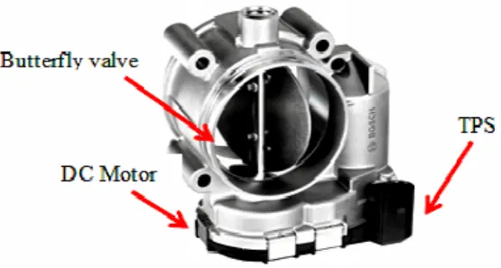
While designing the fuel management system for the SI engine, the amount of air flowing in the cylinders is very important. Performance and emissions can be improved by designing and testing a fuel management system in a computer environment and it can also save valuable setup time in an engine test cell.

Procedure:

1. Import the elbow geometry into the converge studio. Here we have to do the geometry cleanup. The imported elbow has the thickness of the wall. We have to convert the elbow thickness to the flow region to identify the simulation flow. For that, we have to delete the outer face and the 2 thickness faces(input, output) of the elbow. Use the 'By angle' option and select the outer and thickness faces and click D to delete the faces.

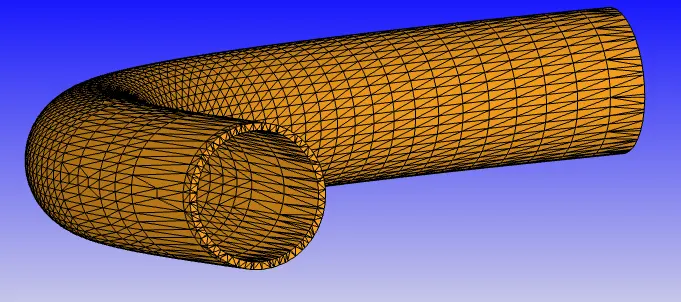
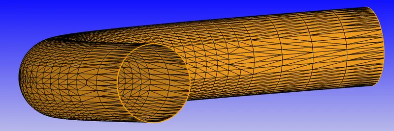
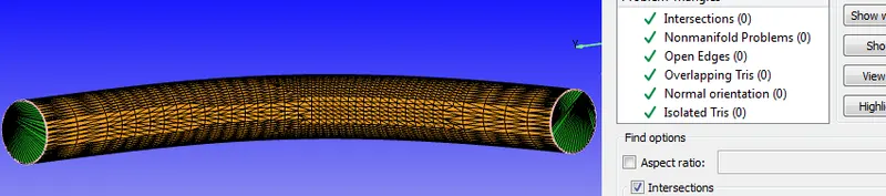
2. Create patch-ups: Now click on diagnosis > Find > then we seen an error in open edges which was shown in below fig. To avoid that click on repair > patch > free edge loop > select the edges one after another > apply.

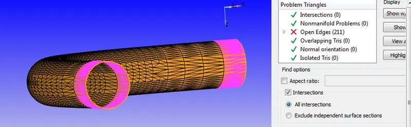
The patch should be formed on both sides of the elbow as shown in the below fig.

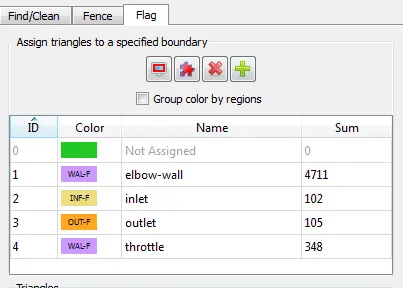
3. Create and assign boundary: Click on boundary > flag > plus icon and create 3 flags and assign the boundary names to it. For throttle hide the elbow and select the throttle.

4. Run diagnosis:

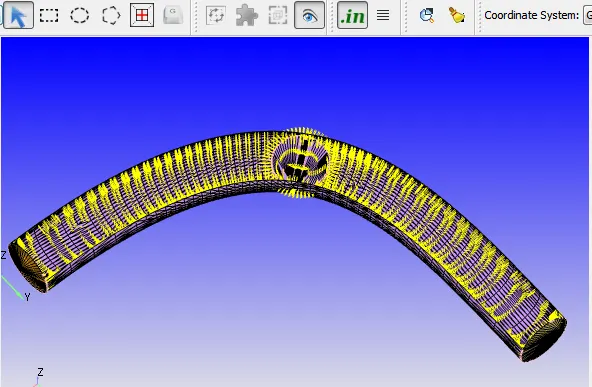
Run the diagnosis to ensure that there should be no errors. Enable the 'check that all normals are pointing to the interior'.

5. Case setup:

5.1 Select a time-based application in the application type.

5.2 Materials: Select air in predefined materials and enable reaction mechanism. And coming to gas simulation global, transport properties and reaction mechanism are set as default values.

5.3 Simulation Parameters:

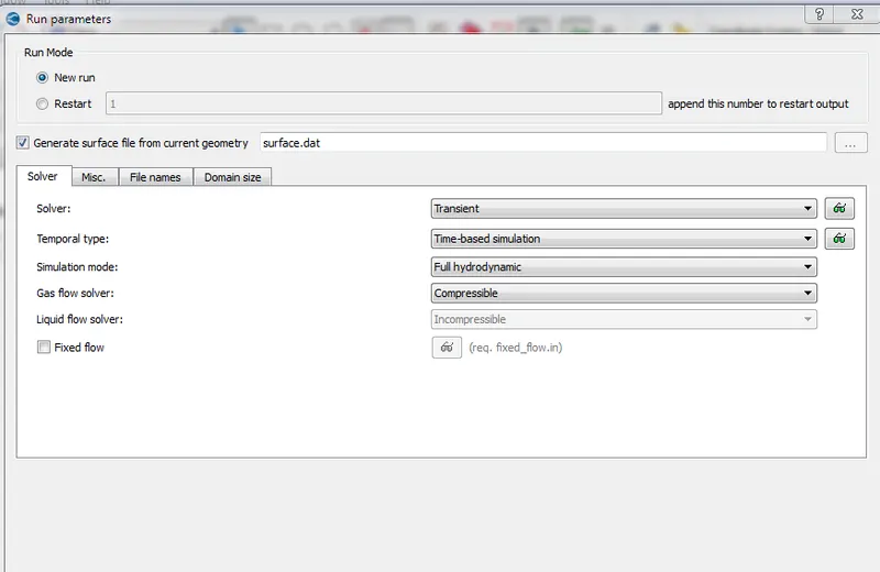
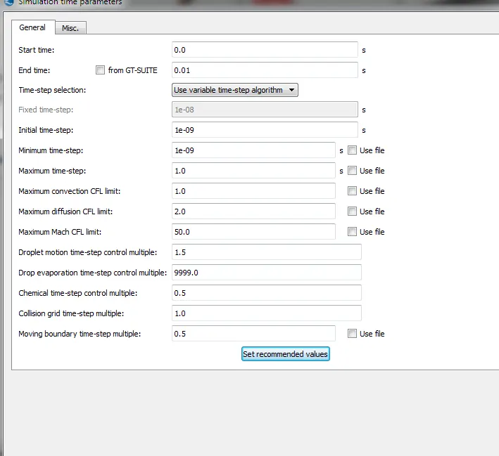
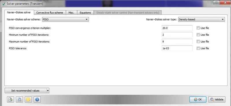
Here we are using a transient solver. So, in time parameters the start and end time should be seen in seconds because of transient solver, while we see cycles in steady-state solver. In solver-parameters use density-based in navier-stokes solver type and remaining all set to default.

5.4 Initial conditions and events:

5.5 Grid control:

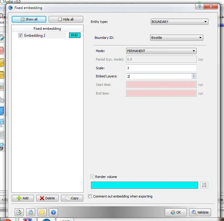
Keep base grid size as dx = dy = dz = 0.002. And select fixed embedding for the throttle.

5.6 Output/post-processing:

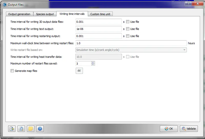
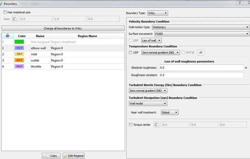
5.7 Boundry conditions:

Elbow wall:

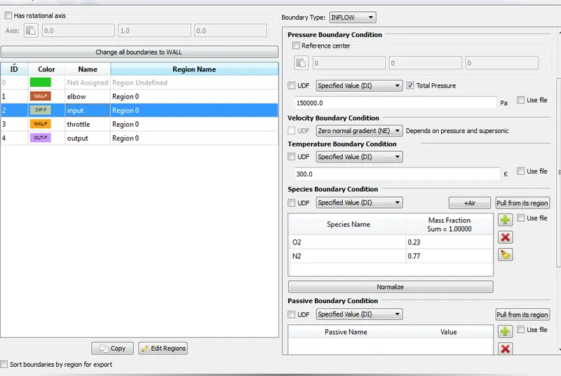
Input:

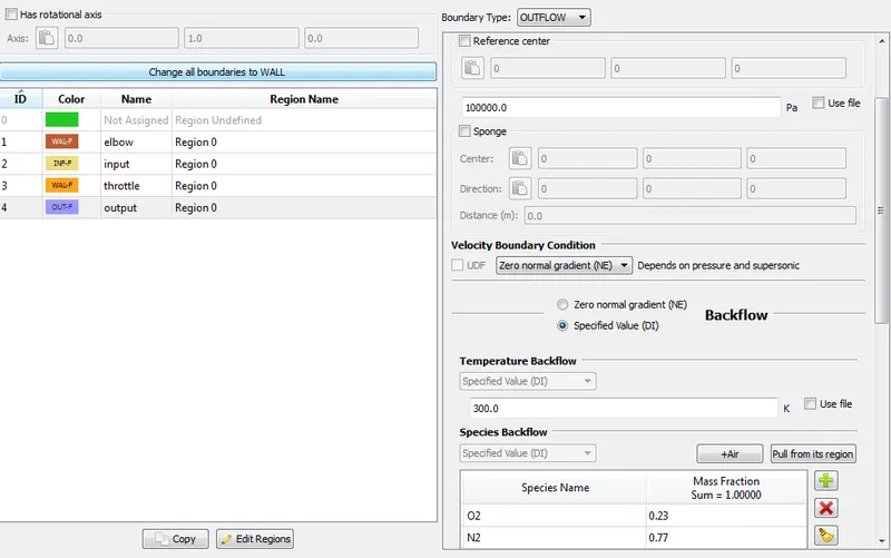
Output:

Throttle:

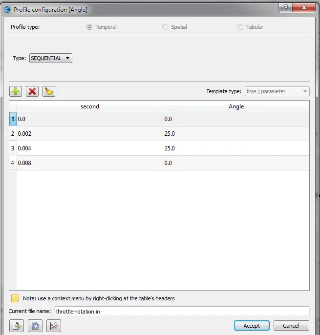
Here we are using a transient state, so the throttle would rotate. So select a moving option in surface movement and a rotation rate file and name it. In the rotation file, we can mention the rotation angles of the throttle will be mentioned as shown below figure.

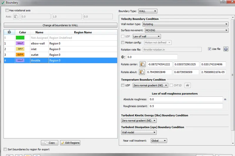
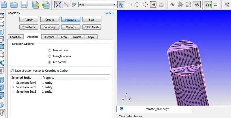
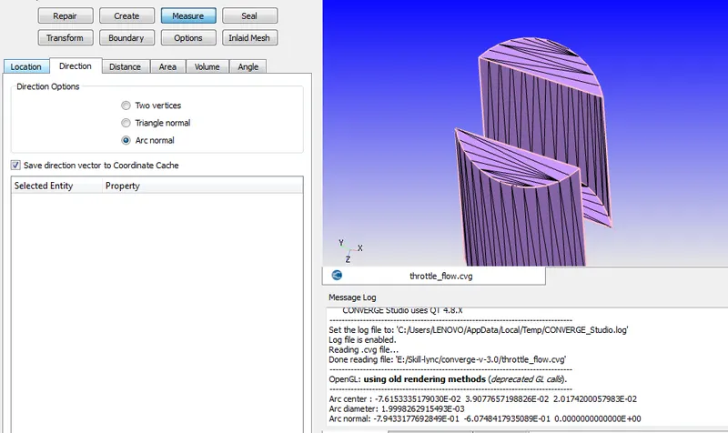
And coming to rotate center and rotate about values are taken from the arc center and arc normal. For the values hide elbow wall > hide walls of the throttle > click on the measure > direction > arc normal > select any 3 on the arc > apply.

6. Now export all input files: Click on files > Export > Export input files > choose the path and select all files and press ok.

7. Run the simulation and post-convert the files: Copy and paste the mpiexec.exe file and converge.exe file to the folder in which the input files are exported to run the simulation in Cygwin. Copy the post_convert_30_msmpi_64.exe file and paste it into the output folder. Now open Cygwin and go to the output folder and type mpiexec.exe -n 4 post_convert_30_msmpi_64.exe > enter the case name(as case1) > select file type as Paraview VTK in-line binary format > type all for files and cell variables and click enter (or) we can convert those files in converge studio.

8. Post-processing the files:

To post-process the files lanch paraview and open the file location as case1 which is saved in output > case1 .. vtm (this is a group file which is formed during post-converting the files) > click on apply > create a slice along the z-axis.

Results:

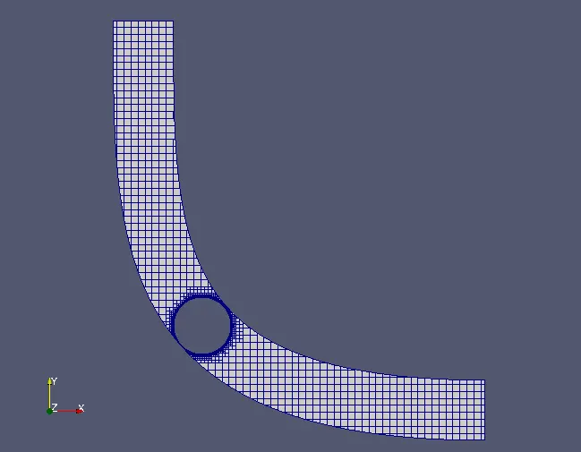
Here we can observe that refined boundary mesh near the throttle boundary and we go away from the throttle body the mesh size gradually increases, this is due to the use of the fixed embedding in the grid control.

Pressure contour at 25 degrees:

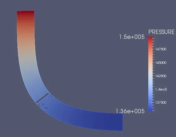
Pressure contour at 0 degrees:

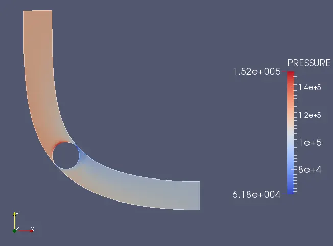
Here the red region(1.4 to 1.5bar) around the throttle shows how the flowing fluid imposes high pressure on the throttle. In the blue region the pressure is low because the flow is constricted.

Velocity contour 25 degrees:

Velocity contour at 0 degrees:

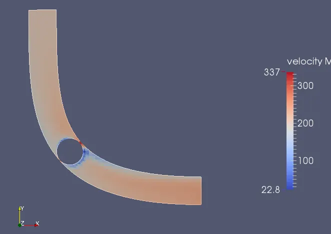
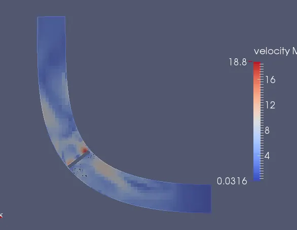
Here on the right side of the throttle, it shows the high velocity(around 337 m/s) in a very small region. The increased velocity is used to maintain the mass flow rate. The blue regions on the top and bottom of the throttle indicate the decrease in the velocity due to the circulation of the throttle.

Plots:

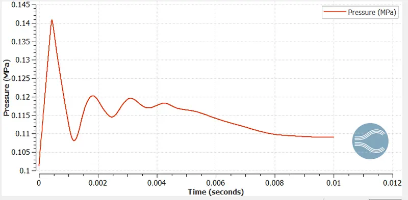
Pressure plot:

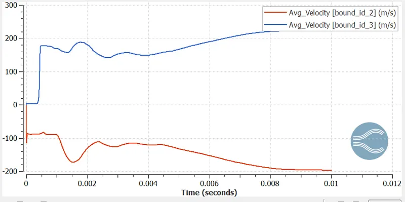
Velocity plot:

Mass-flow rate:

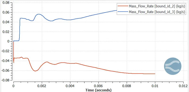
The mass flow rate: 0.066 kg/s

Total cells:

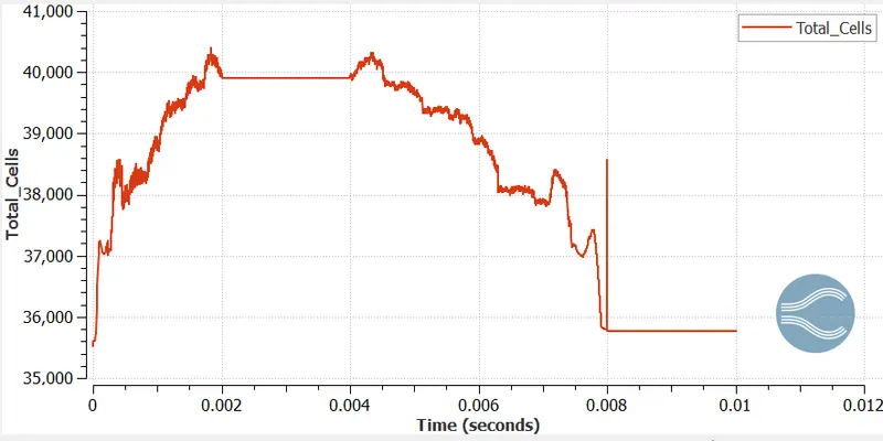
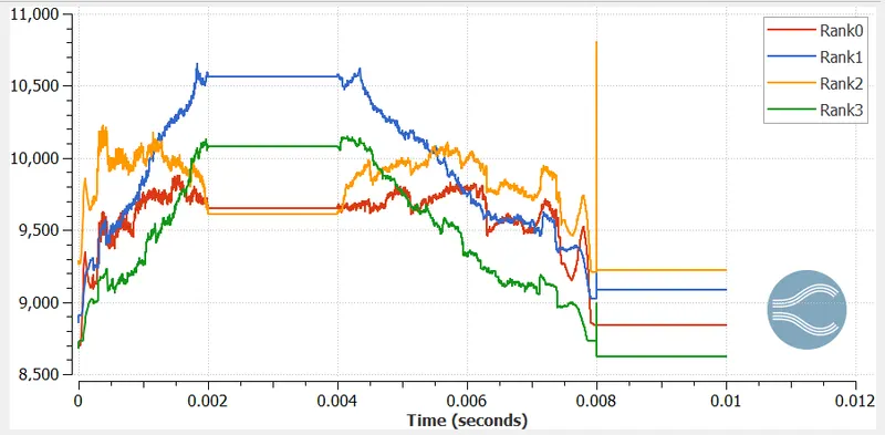
The total cells: Here the throttle rotates from 0 to 25 degrees then the cell count is 40,000. Then again the throttle rotates from 25 to 0 degrees then the cell count will decrease from 40,000 to 35769.

Animation link: https://youtu.be/hCuG26B0DIU

Conclusion:

• In the pressure and velocity contours, there is a variation in 0 and 25 degrees are mentioned.
• The various contour plots of velocity and pressure over a throttle body and the elbow with the changing the throttle angle were analyzed and studied.