Week 4.2: Project - Transient simulation of flow over a throttle body
Aim:
To perform a transient-state flow analysis over a throttle body and draw suitable conclusions.
Introduction :-
In this Transient Simulation, the throttle is rotating and we are interested to simulate the flow at a different opening angle of the throttle.
The main function of a throttle body assembly is to control the airflow into the engine based on vehicle demand. The throttle body is mounted between the air cleaner and the intake manifold. Following the angle of the throttle valve (butterfly valve) changes, it restricts the amount of airflow into the engine cylinder.
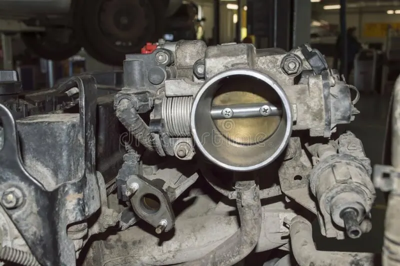
An engine's power can be increased or decreased by the restriction of inlet gases (by the use of a throttle), but usually decreased. The term throttle has come to refer, informally, to any mechanism by which the power or speed of an engine is regulated, such as a car's accelerator pedal. What is often termed a throttle (in an aviation context) is also called a thrust lever, particularly for jet engine powered aircraft. For a steam locomotive, the valve which controls the steam is known as the regulator.
Examples:
1. A hot coffee put in air. (transient heat transfer)
2. Just after switching on a capacitive circuit. (transient voltage-current characteristic in capacitor)
3. An iron piece exposed to carbonaceous environment during surface hardening process. (transient mass transfer)
The variation in the angle of the valve follows the following trend:
- From 0 to 2 ms the valve should rotate by 25 degrees
- From 2 to 4ms it should stay at 25 degrees
- After which by 8ms the valve should get back to it’s original position.
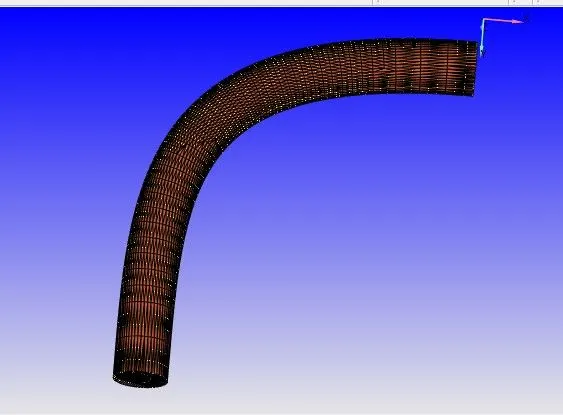
CAD MODEL
Procedure :
To we should do Case setup. Just beside Diagnosis > click on Case setup > in case setup window we can see 'Begin Case Setup" > click on it to see the setup
- Import the Week 4.2.cvg file in converge CFD.
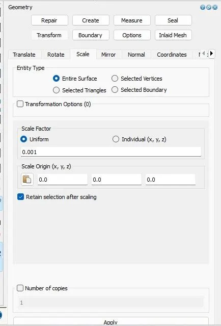
- And scale the geometry from millimetere to meter.
Next go to Geometry > options > select Surface Normal. After selecting the S.Normal the normals point towards outside, so select normal toggle once again then the normal changes their direction to inwards.
After setting the geometry, next important thing is to daignosis the geometry for error/problems. For this go right bottom side, select Diagnosis > click on all intersection > click Find. On top we can check for problems in problems Traingles.
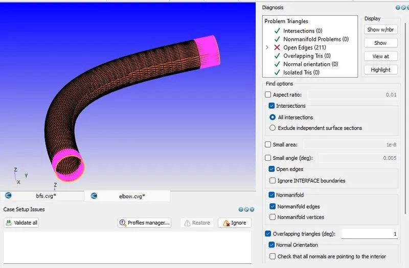
Now if there are no errors found then the geometry is correct.
Creating the boundary face and delete the thickness of the elbow.
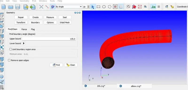
Image - Delete outer Case
After deleting the thickness the open edge is created. Next, the open edge is closed by patch command. Select edge option & select by open edge and go to Repair --> Patch --> patch the inlet & outlet of the component.
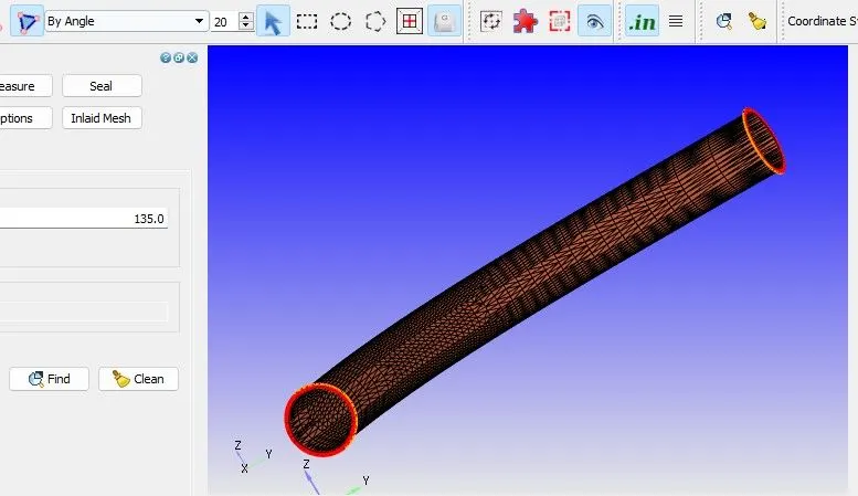
Image - Delete the outer edge and make patches on it
- Go to Boundary --> flag --> make 3 new boundaries.
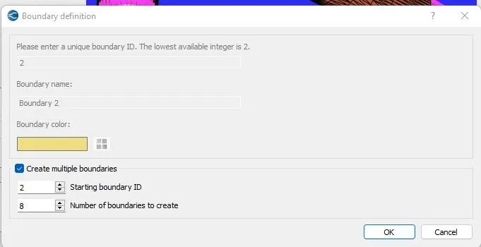
- Go to view option --> hide boundaries in order to Assign boundaries like inlet,outlet.
- Now, hide inlet & outlet boundaries and we will able to see the throttle body.
- Go to Daignosis --> click on clear.
- Click on Box pick [] and draw the mouse to see the component into a half in order to see the throttle.
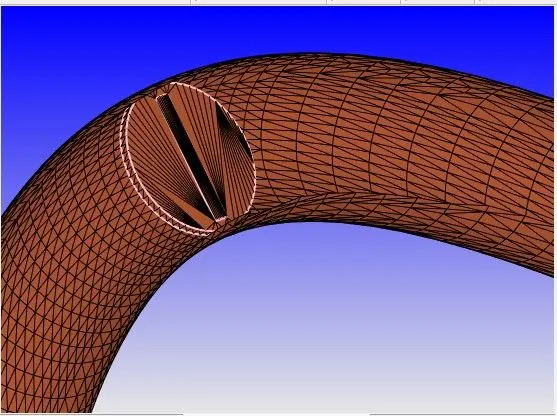
Enable Normal and we can see some of the Normal point outward & some of the inward so but we can do we can simply press Normal Toggle once again and the outward issue is now resolved.
Click on Diagnosis --> Find --> now we can see all problem Traingles are resolved. Now, our boundary flagging is complete.
Next, go to the case setup .
B. Case Setup:-
1. Application Type:- Time -based
2. Material:-
- Use Air as predefined mixtures.
- Enable gas simulation
- Enable reaction meachanism(mech.dat)
3. Simulation Parameters:-
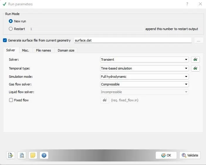
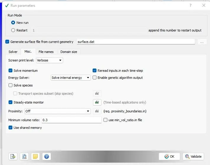
A. Run Parameters
- A Transient solver is used.
- Time-based simulation is picked.
- Hydrodynamic solver is setup.
- Uncheck steady state monitor & UseShareMemory.
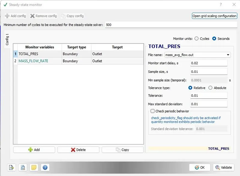
B. Steady State Monitor
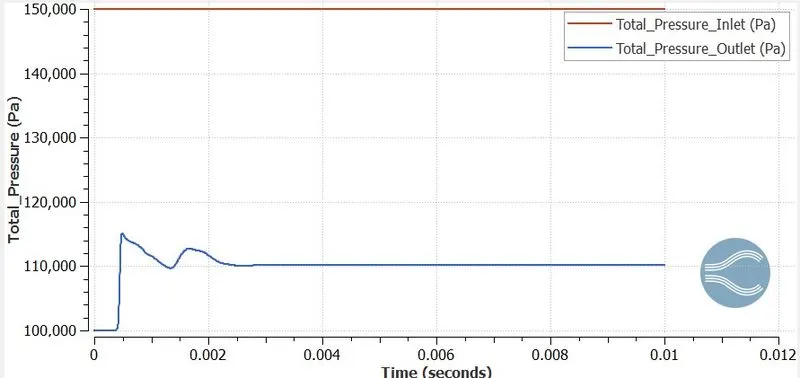
Click on Add and assign two monitor variable Total_Pressure and Mass_flow_rate
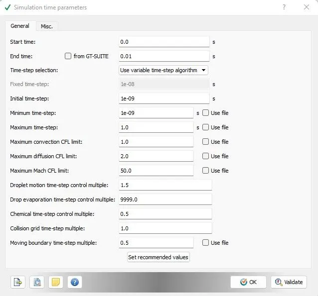
C. Simulation Time Parameters
5. Boundary Conditions:-
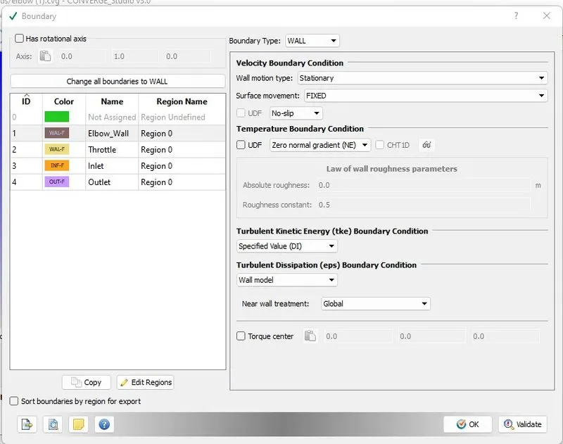
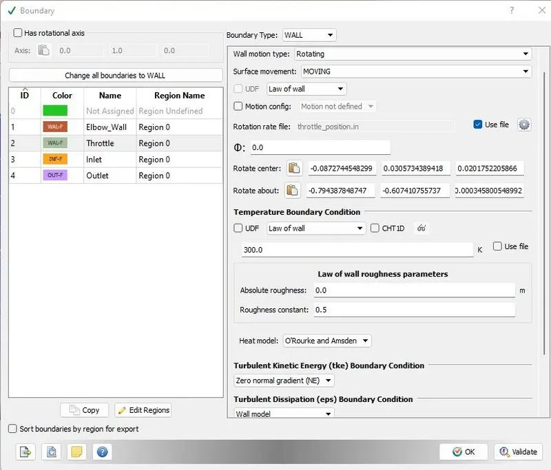
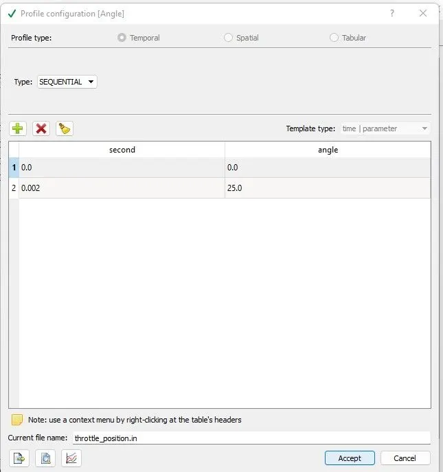
Hide all the other component by clicking on the right bottom 'View Options' and we are not only left with throttle valve and then
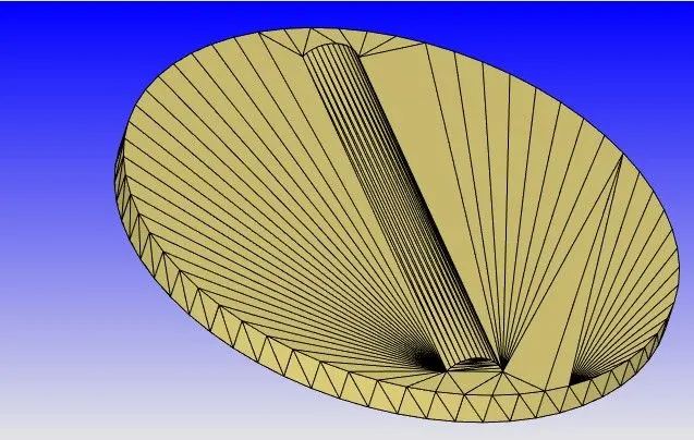
next hide the other parts by clicking right button of the mouse and hide selection there as shown in the given figure as shown in the given below figure.
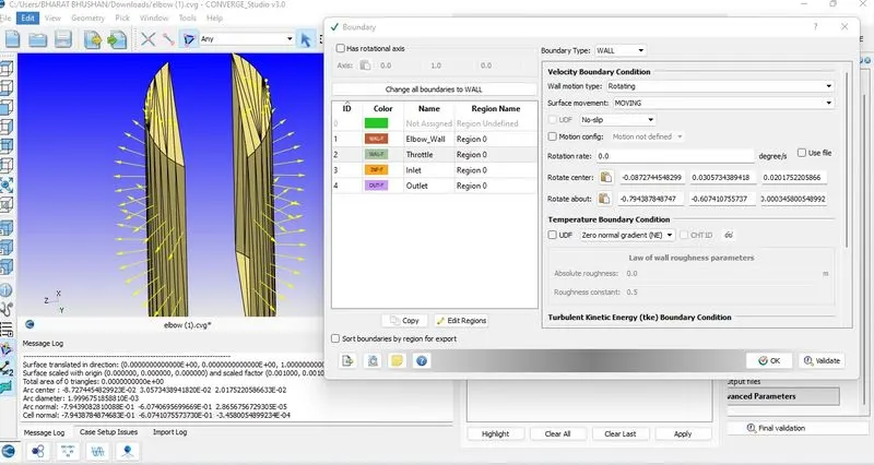
So we have to fill the value of 'Rotate Center' and 'Rotate about' so for that
Go to --> Geometry --> Measure --> Direction --> Arc normal and select the 3 points correspondingly and click on Apply so we will get the value of Arc normal.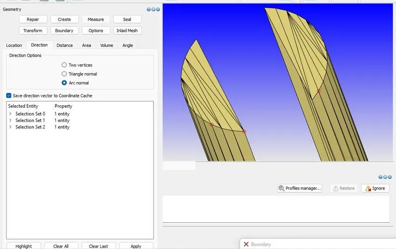
So paste the value of Arc normal from the 'Message log' and paste into the box of 'Rotate about'.
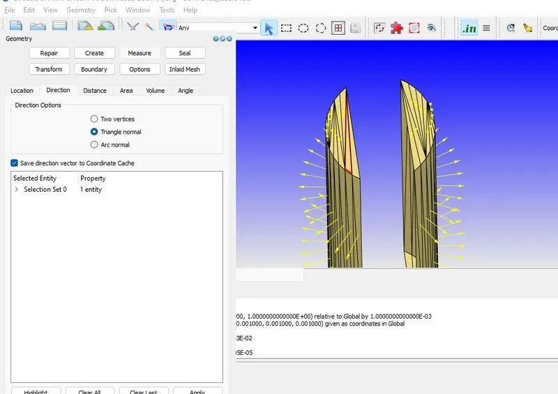
Next, Go to --> Measure -> Direction --> Triangle normal and select any traingle of the given figure and click on Apply and we will get the value of 'Cell normal' and paste into the 'Rotate about' in the Throtte_valve box.
6. Region and Initialization:-
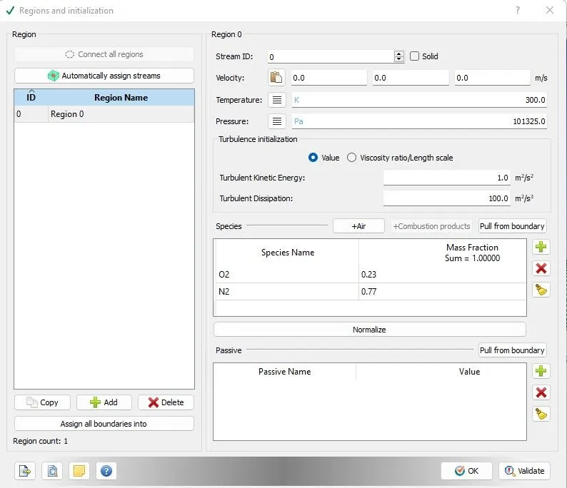
Here click on Add and Assign the Region
7. Grid Control :-
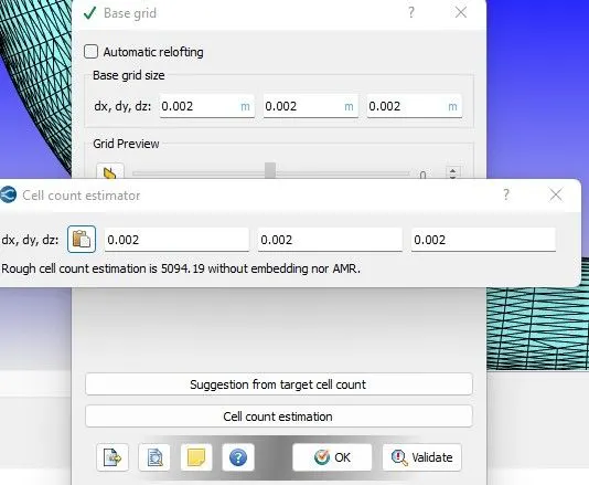
Base Grid
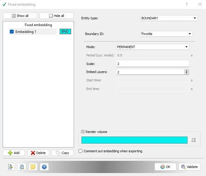
Fixed Embedding
8. Output Files :-
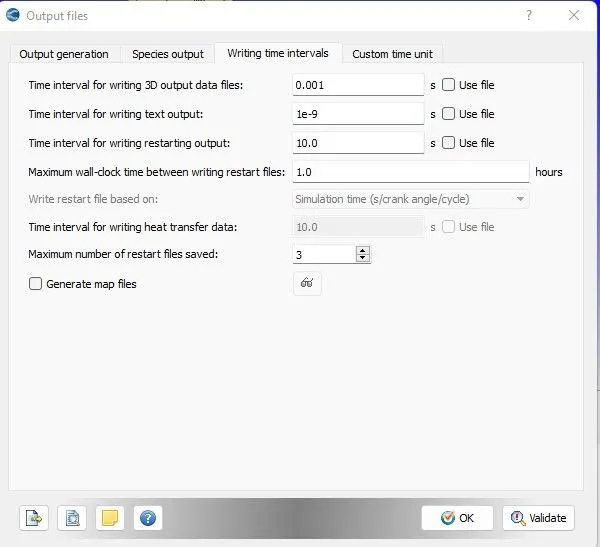
Output files_Writing time intervals
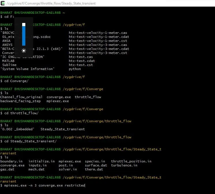
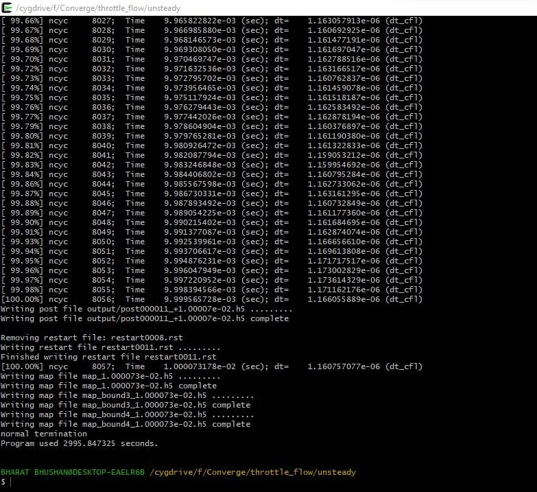
So next export all the input Files to the desire loction folder and Run the simulation in the CYGWIN.
Next, Move to the Plotting section
PLOTS :-
Average Velocity Plot
Mass Flow Rate Plot
Total Pressure Plot
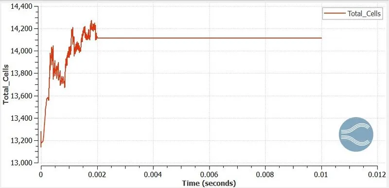
Total Cell Count Plot
After plotting these all move to the post processing
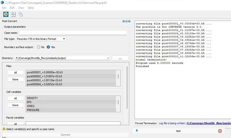
then next i am going to launch the paraview to make Animation and few contours.
CONTOURS:-
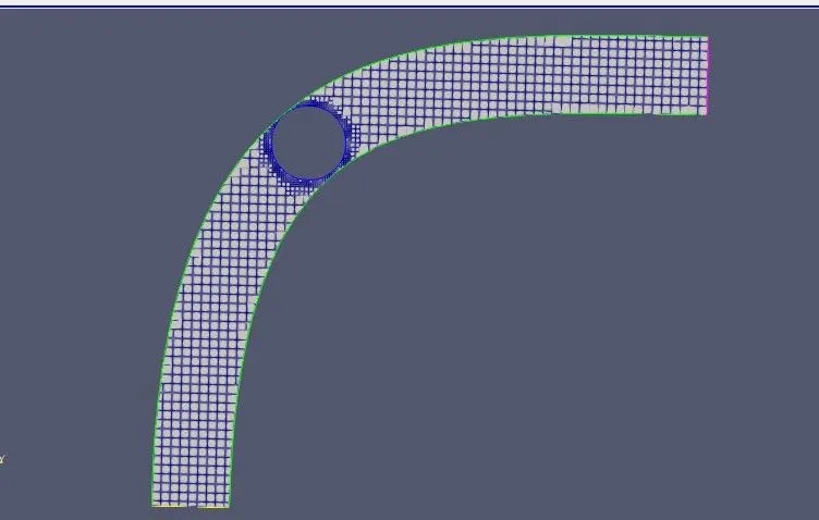
Mesh Grid Contour
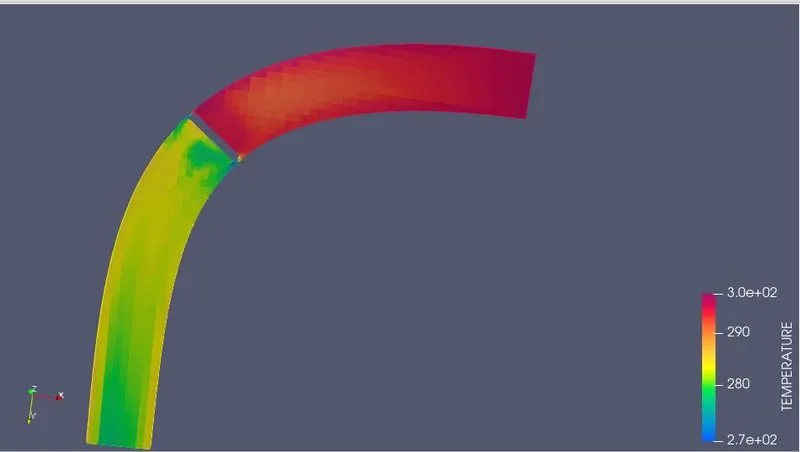
Temperature_Contour
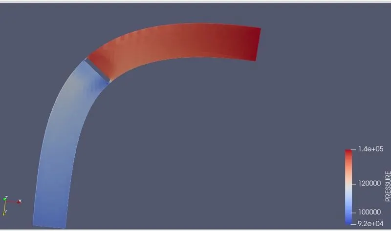
Pressure_Contour
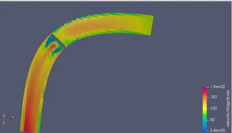
Velocity_Contour
ANIMATION :-
Temperature_Animation
Pressure_Animation
Velocity_Animation
Results :-
From the above contours it is clear that, on giving the finer mesh to the valve the contours appear more detail and the results are highly accurate.
The flow through the throttle position is more accurate as the mesh genereted along the throttle position is refined (having more cells surrounding the valve) i.e by providing 2 embedded layers and a scaling of 2 to the mesh.
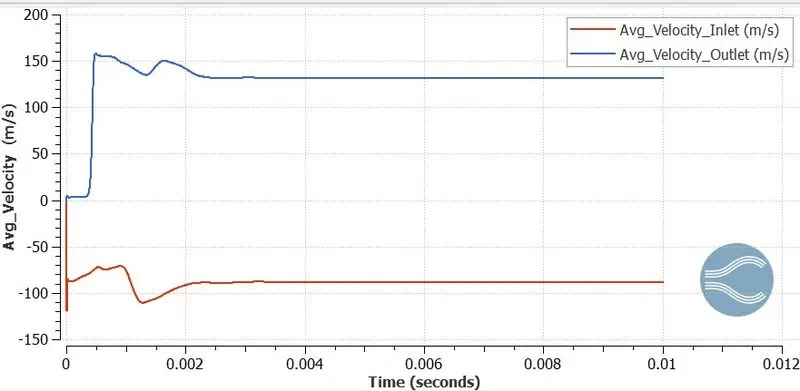
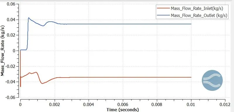
The contours show that, there is a restriction to the flow of intake air that is caused by throttle plate. The inflow mass flow rate is balanced by the outflow rate.
If there is less restriction in the flow, then there is a lower loss in energy. Hence because of this the velocity at outlet increases.
As we having a moving mesh, number of cells generated are more and hence simulation time is high.
Google drive link of file :
https://drive.google.com/file/d/16Qq3JdI2mvnt46v9nvjSBxYT9Hg07kKy/view?usp=sharing