Week 4.2 - Curve fitting

Aim:

• Write the code required cubic and linear polynomials to fit the Cp (Specific Heat) data.

Objective:

• To write the code to fit a linear and cubic polynomial for the Cp data.
• Plot the linear and cubic fit curves along with the raw data points.
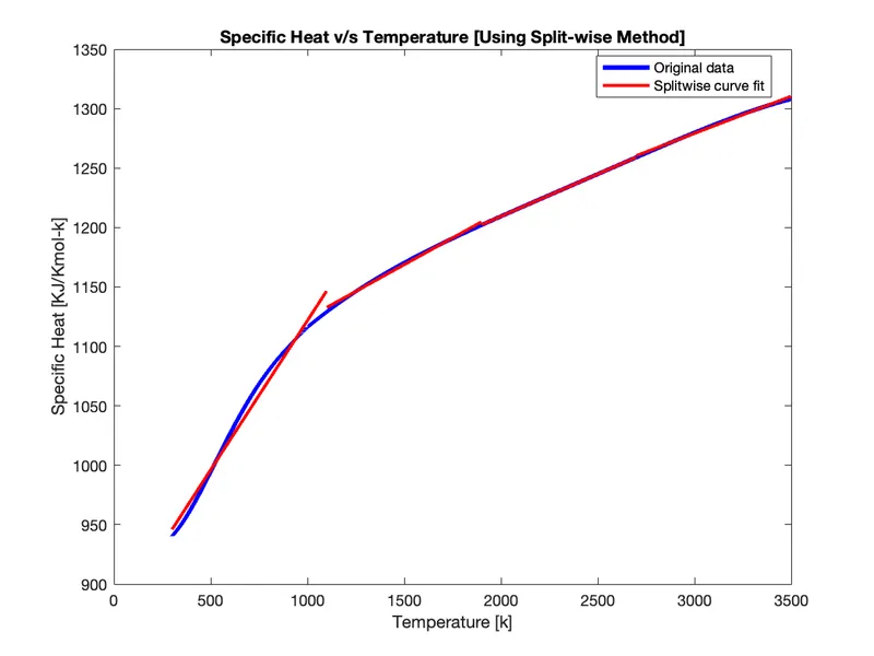
• To write a code to show the splitwise method
• To explain the parameters used to measure the fitness characteristics for both the curves,

FACTORS ENTAILED:

Curve Fitting:

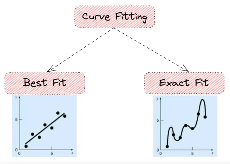
• One of the most potent and frequently employed analytical tools is curve fitting. In order to identify the "best fit" model of the relationship, curve fitting examines the correlation between one or more predictors (input variables) and a response variable (dependent variable). Linear and polynomial fits are the two most common types of curve fits.

• In curve fitting, a function called f(x) must first be approximated using a simpler function, such as a polynomial, a trigonometric function, an exponential function, or a rational function. The primary distinction between interpolation and curve fitting, however, is that in the former, the approximated curve must traverse the provided data points. Once more, polynomial functions are those that are utilised more frequently in applications than other functions.

• Using interpolation, you can find a function that perfectly fits the data points. This has limited applicability to real-world situations because it makes no assumptions about measurement error. When we find a function that roughly fits the data points, we smooth it out by allowing for some error and allowing the actual data points to be close to, but not exactly on, the line. This is done as long as the overall amount of error is kept to a minimum.

Linear and Polynomial Curve fitting :

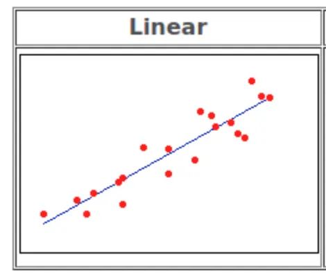
• Linear curve fitting, or linear regression, is when the data is fit to a straight line. Although there might be some curve to your data, a straight line provides a reasonable with enough fit to make predictions.
• cp = a*t+b
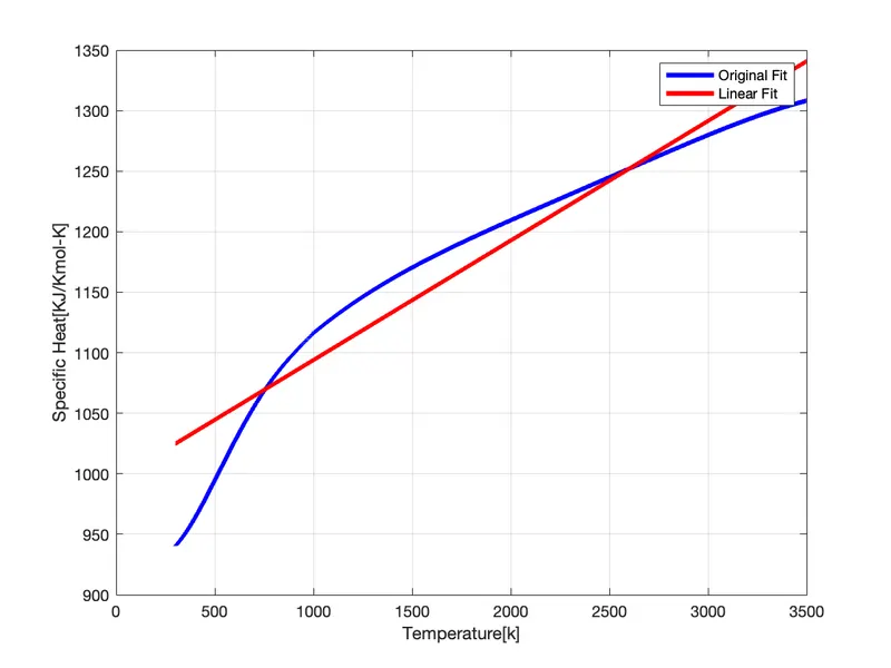
• Coefficients of a linear polynomial is determined by the command 'co_effs_linear = polyfit (temperature,cp,1)'. In this, the 'temperature' and 'cp' are the variables involved in the polynomial and '1' is the order of the polynomial. 'Cp' values are predicted with the help of the command 'predicted_cp_linear = polyval(co_effs_linear,temperature)'.

• We can express how far from "best" the prospective line is by taking the vertical distance between each point and the line as an error and adding those distances across our range. The best straight line is one that has the least amount of error.

• We square the distance in our error calculations because the distance between our points and the line is what we're interested in—whether it's a positive or negative distance is unimportant. Additionally, it enables us to give bigger errors more weight. So the least squares approach is the name given to this method. SSE is calculated for the linear fit.

Cubic Fit :

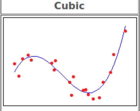
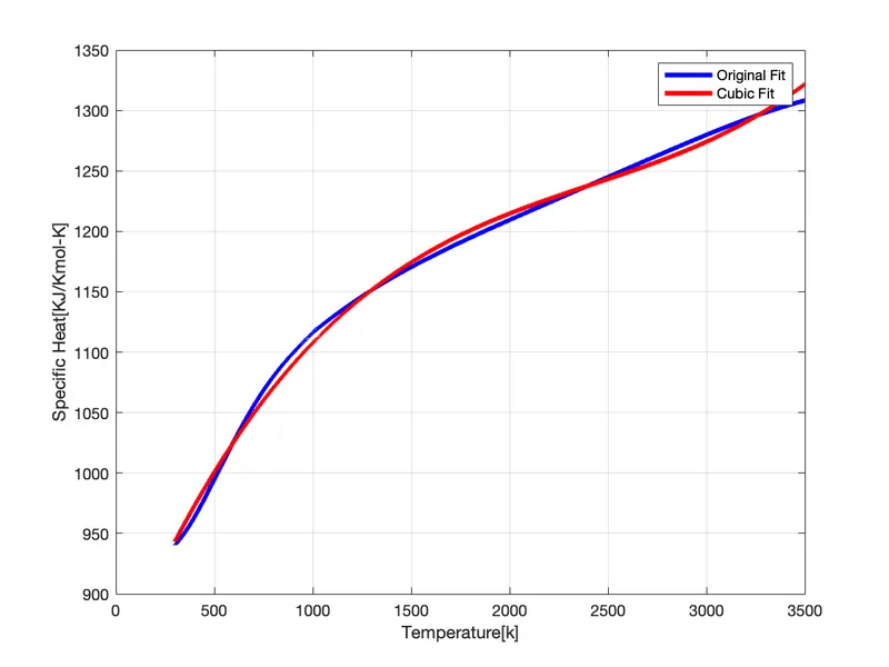
• coefficients of a cubic polynomial is determined by the command 'co_effs_cubic = polyfit(temperature,cp,3)'. In this, the 'temperature' and 'cp' are the variables involved in the polynomial and '3' is the order of the polynomial. 'Cp' values are predicted with the help of the command 'predicted_cp_cubic = polyval(co_effs_cubic,temperature)'.
• cp = a*t^3+ b*t2 + c*t+d

• Cubic fit is plotted with temperature on the x-axis and predicted values of cp on the y-axis. Measuring the fitness characteristics of the curve:

• The Sum of squared errors is a criterion to measure the goodness of fit or how well the equation represents the data points. SSE is calculated for the Cubic fit.

Matlab Program:

• For linear curve fit,

close all
clear all
clc

%Step 1: Preparing the data

cp_data = load('data');
temperature = cp_data(:,1);
cp = cp_data(:,2);

%Step2: Plotting the Original datafigure(1)

plot(temperature,cp, 'linewidth',3,'color','b')
xlabel('Temperature[k]')
ylabel('Specific Heat[KJ/Kmol-K]')
grid on

%Step3: Curve Fitting

%Linear Fit

%cp = a*t+b 

co_effs_linear = polyfit(temperature,cp,1);
predicted_cp_linear = polyval(co_effs_linear,temperature);

%Plotting linear fit

plot(temperature,cp,'linewidth',3,'color','b')
hold on
plot(temperature,predicted_cp_linear,'linewidth',3,'color','r')
xlabel('Temperature[k]')
ylabel('Specific Heat[KJ/Kmol-K]')
legend('Original Fit','Linear Fit')
grid on

%Cubic Fit

%cp = a*t^3+ b*t2 + c*t+d

co_effs_cubic = polyfit(temperature,cp,3);
predicted_cp_cubic = polyval(co_effs_cubic,temperature);

%Plotting Cubic fit

plot(temperature,cp,'linewidth',3,'color','b')
hold on
plot(temperature,predicted_cp_cubic,'linewidth',3,'color','r')
xlabel('Temperature[k]')
ylabel('Specific Heat[KJ/Kmol-K]')
legend('Original Fit','Cubic Fit')
grid on

%Step4: Measuring of the Fitness Characteristics of the curves

Error_linear = cp - predicted_cp_linear;
Squared_Error_linear = Error_linear.^2;

%SSE = Sum of Squared ErrorsSSE_linear = sum(Squared_Error_linear);

Error_cubic = cp - predicted_cp_cubic;
Squared_Error_cubic = Error_cubic.^2;

%SSE = Sum of Squared ErrorsSSE_cubic = sum(Squared_Error_cubic);

• For cubic curve fit OUTPUT,
• 
• The splitwise method Matlab program,

clear all
close all
clc
%Distinguish The Data Sheet

cp_data = load('data');
tempr = cp_data(:,1);
cp = cp_data(:,2);

% Curve Fit 

%using splitwise Method

a = 1;
b = 3200/4;

%Using For Loop

for i = 1:4
   temp(:,i) = tempr(a:b);
   
   
% cp1 = a*temp + b | Linear Polynomial

co_effs1= polyfit(tempr(a:b), cp(a:b),1);
predicted_cp1 = polyval(co_effs1,tempr(a:b));


 % For Quality of Fit  | SST = SSR + SSE
  
SSR = sum((predicted_cp1 - mean(cp)).^2);    %sum of sq of regression
SSE = sum((cp(a:b) - predicted_cp1).^2);     %sum of sq error
SST = SSR + SSE;                    

%Goodness OF Fitting | R_sq = (SSR/SST)

R_sq(i) = (SSR/SST);


a = b + 1;
b = b + 3200/4;


  predicted_cp1_new(:,i)= predicted_cp1;
  
 
end 

 %plot  

  plot(tempr,cp,'linewidth',3,'color','b')
  hold on
  plot(temp(:,1),predicted_cp1_new(:,1),'linewidth',2,'color','r')
  plot(temp(:,2),predicted_cp1_new(:,2),'linewidth',2,'color','r')
  plot(temp(:,3),predicted_cp1_new(:,3),'linewidth',2,'color','r')
  plot(temp(:,4),predicted_cp1_new(:,4),'linewidth',2,'color','r')
  xlabel('Temperature [k]')
  ylabel('Specific Heat [KJ/Kmol-k]')
  legend('Original data' , 'Splitwise curve fit ')
  title('Specific Heat v/s Temperature [Using Split-wise Method]')

  
%Quality of fit R-squared(R_sq) = SSR/SST 

%For Linear Polynomial using Split-wise method

R_square = mean(R_sq(i));

• Split wise Fitting OUTPUT;

Based on the research, the answer to the following questions are:

1. How to make a curve fit perfectly?

• By increasing the order of the polynomial, the predicted data curve moves closer to the original data curve, allowing us to make a curve fit perfectly.

2. How to get the best fit?

• There are four factors that help us gauge the goodness of fit of a curve after we locate one that fits the data.
• The sum of Square due to Error (SSE)
• R-square
• Adjusted R-square
• Root mean Squared Error (RMSE).

3. What could be done to improve the cubic fit?

• By dividing the curve over the actual data, we can use the split wise and fit the curve. We can create a programme that asks the user for the number of splits so that the best fit can be determined after splitting.

Conclusion:

• Resultantly, we can draw the conclusion that a good curve fit, R2R2 should be close to 1. The results show that theR2R2for the linear curve fit is approximately 0.93, and theR2R2for the cubic curve fit is almost 0.99. Therefore, cubic polynomials fit the data better than linear polynomials. The value ofR2R2will move closer to 1 as the polynomial's order rises, and the fit will be considered to be sufficient.

Reference:

• https://skill-lync.com/student-projects/Curve-Fitting-and-criterion-to-choose-best-fit-41860
• https://engineering.vanderbilt.edu/ge/es140/Otherlinks/MatlabTutorial/CurveFitting.php
• https://in.mathworks.com/help/matlab/ref/polyfit.html