Week 4.1 - Solving second order ODEs

Main Program

%%
clear all;
close all;
clc

%% Introduction 
fprintf('\n');
disp('In this challenge we are going to plot the "ANGULAR VELOCITY & DISPLACEMENT" of a simple pendulum with respect to time, using second order differential equation');
fprintf('\n');
disp('Here is the equation');
fprintf('\n');
disp('(d^2theta/dt^2)+(b/m)(dtheta/dt)+(g/l)sin(theta)=0');
fprintf('\n');
disp('Where b is damping co-efficient, m is mass of ball, l is length of pendulum & g is gravitational constant which is universal 9.81 m/s^s');
fprintf('\n');
disp(' In this problem all the coefficient values has been given');
fprintf('\n');
disp('b=0.05');
disp('l= 1 metre');
disp('m=1 kg');
disp('g=9.81 m/s^2');

%% Assigning values
b=0.05;
m=1;
l=1;
g=9.81;

%% Declaring initial conditions
theta_0=[0;3]  % The angular velocity has been given as 3 rad/sec at time t=0
t_span=linspace(0,20,300);  % The time span has been mentioned from 0 to 20 seconds

%% Calling the inbuilt solver ODE45
[t, results]=ode45(@(t,theta) ode_func(t,theta,b,g,l,m),t_span,theta_0); % Here time t is independent variable & theta is dependent of t

%% Plotting the results of angular displacement and angular velocity with respect to time t
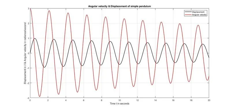
plot(t,results(:,1),'linewidth',1.5,'color','k'); % Plot of displacement
hold on
plot(t,results(:,2),'linewidth',1.5,'color','r'); % Plot of angular velocity
grid on
title('Angular velocity & Displacement of simple pendulum');
axis([0 20 -3 3]);
xlabel('Time t in seconds');
ylabel('Displacement in \theta & Angular velocity in radiance/second');
legend('Displacement','Angular velocity');

%% Counter for animation
ct=1;

%% Creating animation of a simple pendulum
for i=1:length(results(:,1)) % considering the displacement array as index value  
    X0=0;                    % fixed point for pendulum
    Y0=0;                    
    L=1;                     % Length of pendulum rope
    X1=L*sin(results(i,1)); 
    Y1=-L*cos(results(i,1)); 
    figure(2) 
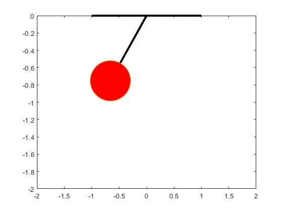
    plot([X0 X1],[Y0 Y1],[-1 1],[0 0],'linewidth',3,'color','k')  %plotting the pendulum string 
    hold on 
    plot(X1,Y1,'o','MarkerSize',60,'Markerfacecolor','r')         % plotting the pendulum bob 
    axis([-2 2 -2 0]); 
    pause(0.03)                                                   % This command pauses the animation for 0.03 seconds
    hold off  
    f(ct)=getframe(gcf);                                         % Captures the each frame of the figure as per the length of array
    ct=ct+1;                                                     % The counter value gets incremented by 1, when "for" loop runs each & everytime
end 

%% Making movie from above animated plot
movie(f,2,12); % This command plays the movie 2 times at the rate 12 frames per second
videofile=VideoWriter('pendulum_simulation.avi','Uncompressed AVI'); % Creates an object in AVI format
open(videofile); 
writeVideo(videofile,f); 
close(videofile);

Function Code

function [dtheta_dt]=ode_func(t,theta,b,g,l,m)

theta1=theta(1);
theta2=theta(2);
dtheta1_dt=theta2; % The entire second order ODE has been reduced to two first order ODE's 
dtheta2_dt=(-b/m)*theta2-((g/l)*sin(theta1));
dtheta_dt=[dtheta1_dt;dtheta2_dt];

end

Output Plots

Error messages

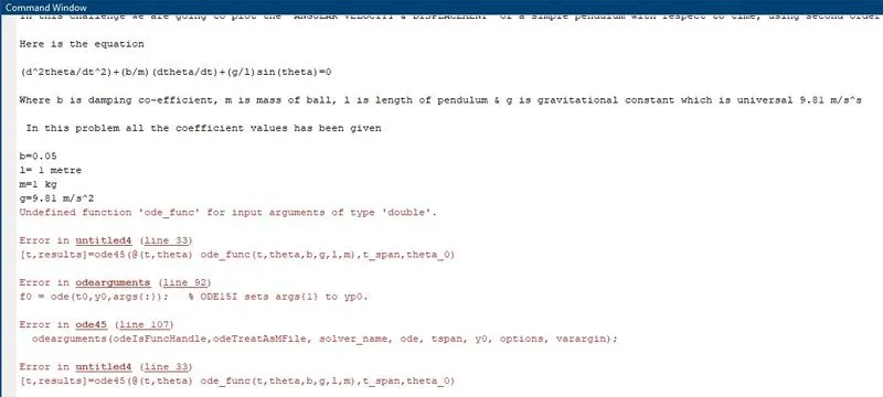
1) Error in arguments - The error was due to improper declration of arguments or variables b, g,l &m. The sequence in which they were declared was not same in main program code & function code

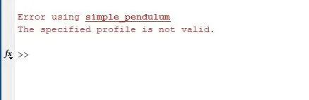
2) The arguments inside the PLOT command was not declared properly, due to which it throwed a error

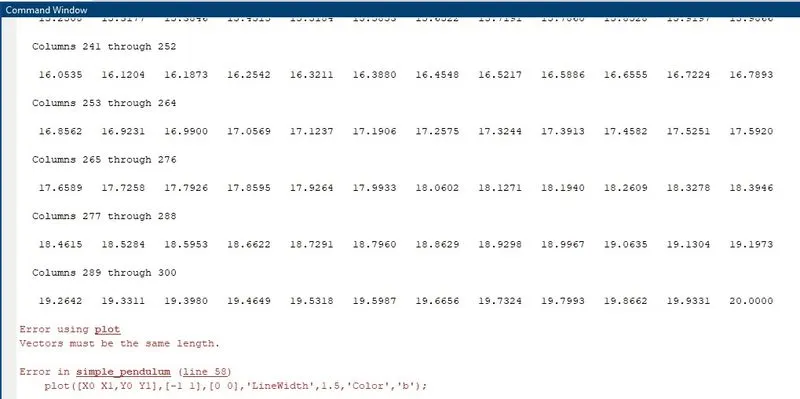
3) Interruption occured when program was under RUN mode