Week 4.1 - Solving second order ODEs
Simulation video link:-
https://drive.google.com/file/d/1GlZf2z0W_o7u0_4XckLx3nSH9yZqRRK3/view?usp=sharing
Aim:
To solve second order ordinary differential equation using MATLAB.
Objective:
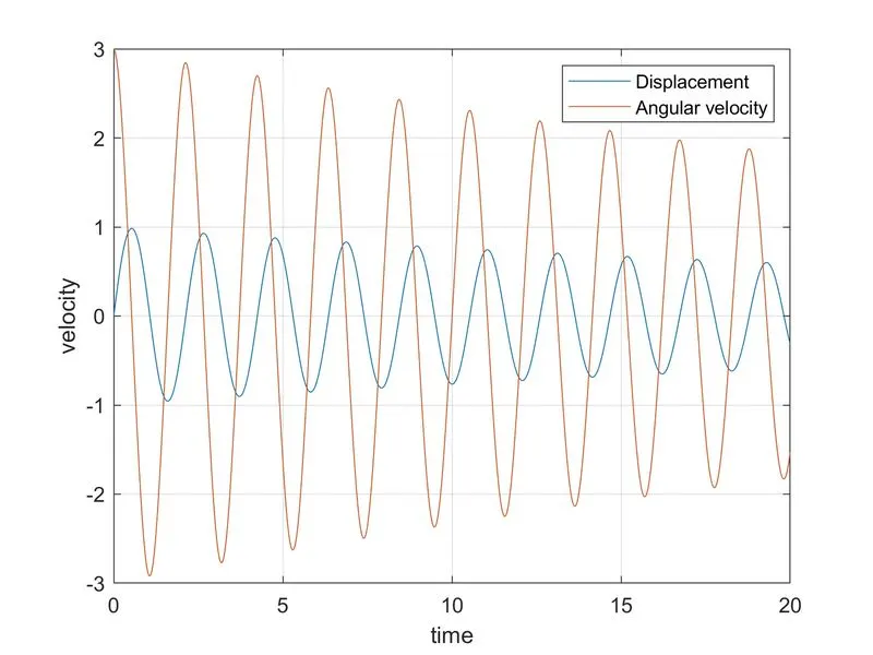
1-To solve the second order ODE with graph of Velocity v/s Displacement.
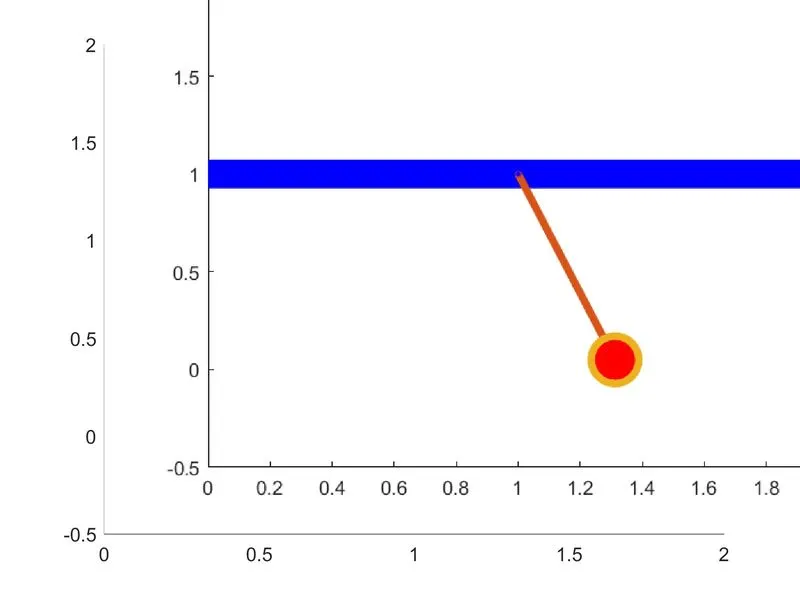
2-To create the animation of the simple pendulum.
clear all
close all
clc
% inputs
b=0.05;
g=9.81;
l=1;
m=1;
% initial condition
theta_0 = [0;3];
% time points
t_span = linspace(0,20,500);
% solve ODE
[t,results] = ode45(@(t,theta) ode_func(t,theta,b,g,l,m),t_span,theta_0);
figure(1)
plot(t,results(:,1))
hold on
plot(t,results(:,2))
xlabel('time')
ylabel('velocity')
figure(1)
hold on
legend('Displacement','Angular velocity')
grid on
hold off
displacement = results(:,1);
velocity=results(:,2);
%fixed coordinates
x0=1;
y0=1;
ct=1;
for i = 1:length(displacement)

%coordinates
x1=1-l*sin(displacement(i));
y1=1-l*cos(displacement(i));

figure(2)
%plot fixed link
plot([0 2],[1 1],'linewidth',15,'color','b')
hold on
plot([1 x1],[1 y1],[x1 x1],[y1 y1],'-O','markersize',25,'markerfacecolor','r','linewidth',4)
plot(x0,y0,'-O','markersize',3,'markerfacecolor','b')
%axis setting
axis([0 2 -0.5 2])
hold off
M(ct)= getframe(gcf); % to change the frame of the movie
ct=ct+1;
end
movie(M) %for creating animation video
Videofile=VideoWriter('simple pendulum.avi','uncompressed AVI');
open(Videofile) %open the videofile while running the code
writeVideo(Videofile,M) %for writing the video file
close(Videofile) %for closing the videofile after code run


function [dtheta_dt] = ode_func(t,theta,b,g,l,m)
theta1 = theta(1);
theta2 = theta(2);
dtheta1_dt = theta2;
dtheta2_dt = -(b/m)*theta2 - (g/l)*sin(theta1);
dtheta_dt = [dtheta1_dt; dtheta2_dt];
end
Code explanation:
1-Write a command for clear the workspace, close the previous plot or figure and clear the command window data.
2-Then time span of the simple pendulum is set by using linspace command then,theta value is given as a column matrix.After this we use ode45 function and corresponding 'ode_func' function.
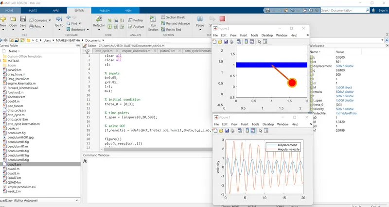
3-The used plot command to plot graph corresponding to time and velocity, legend command is used for identify each values in the graph.
4-For getting the accurate simulation of the simple pendulum corresponding to the second order ODE with damping we need to use the looping statements, here for loop is used to create this.
5-Marker command is used for making bob of the pendulum. The axis is fixed using axis command. The counter command is used to make the value changes in each for loop.
6-Use the getframe command to get individual frame and stored in variable M.
7-The end command is used to end the for loops.
8-Movie command we can create with the help of individual frame.
9-Different individual frames a new uncompressed AVI file is created using video file command.
10-We are opening the videofile using the open command.
11-Closing the videofile using close command.
Theory:
An ordinary differential equation is a differential equation containingone or more functions of one independent variable and the derivatives of those functins. The term ordinary is used in contrast with the term partial differential equation which may be with respect to more than one independent variable.
The simple pendulum is an idealized mathematical model of a pendulum.This is a weight on the end of a massless cord suspended from a pivot,without friction. When given an initial push,it will swing back and forth at a constant amplitude.
The point from which the bob is suspended is known as point of suspension. Weight of the bob acts vertically downwards and the tension acts vertically upwards and the bob starts oscillating if even smaller external force is applied.
for loop:
A loop in general,refers to anything whose start and end points are connected. That is once you begin from the start point a proceed further,you will reach the finish line just to find that it once again guides you to the same point where you started.Proceeding further means that you are repeating your same action again & again.
clear all
close all
clc
% inputs
b=0.05;
g=9.81;
l=1;
m=1;
% initial condition
theta_0 = [0;3];
% time points
t_span = linspace(0,20,500);
% solve ODE
[t,results] = ode45(@(t,theta) ode_func(t,theta,b,g,l,m),t_span,theta_0);
figure(1)
plot(t,results(:,1))
hold on
plot(t,results(:,2))
xlabel('time')
ylabel('velocity')
figure(1)
hold on
legend('Displacement','Angular velocity')
grid on
hold off
displacement = results(:,1);
velocity=results(:,2);
%fixed coordinates
x0=1;
y0=1;
ct=1;
for i = 1:length(displacement)
%coordinates
x1=1-l*sin(displacement(i));
y1=1-l*cos(displacement(i));
figure(2)
%plot fixed link
plot([0 2],[1 1],'linewidth',15,'color','b')
hold on
plot([1 x1],[1 y1],[x1 x1],[y1 y1],'-O','markersize',25,'markerfacecolor','r','linewidth',4)
plot(x0,y0,'-O','markersize',3,'markerfacecolor','b')
%axis setting
axis([0 2 -0.5 2])
hold off
M(ct)= getframe(gcf); % to change the frame of the movie
ct=ct+1;
end
movie(M) %for creating animation video
Videofile=VideoWriter('simple pendulum.avi','uncompressed AVI');
open(Videofile) %open the videofile while running the code
writeVideo(Videofile,M) %for writing the video file
close(Videofile) %for closing the videofile after code run
function [dtheta_dt] = ode_func(t,theta,b,g,l,m)
theta1 = theta(1);
theta2 = theta(2);
dtheta1_dt = theta2;
dtheta2_dt = -(b/m)*theta2 - (g/l)*sin(theta1);
dtheta_dt = [dtheta1_dt; dtheta2_dt];
endConclusion:
1-The graph of Displacement and Angular velocity is plotted in velocity v/s Time diagram.
2-Animation of simple pendulum is created.