Week 4.1 - Solving second order ODEs
AIM: To write a program to solve the ODE which represents the equation of motion of a simple pendulum with damping and create an animated video of outputs obtained by solving the ODE
THEORY: A simple pendulum consists of a mass m hanging from a string of length L and fixed at a pivot point P. When displaced to an initial angle and released, the pendulum will swing back and forth with periodic motion. By applying Newton's second law for rotational systems, the equation of motion for the pendulum may be obtained
where, b = damping coefficient
m = mass of the ball in Kg
L = length of the pendulum in meter
g = gravity in m/s^2
The above equation is a second-order differential equation. The fundamental idea behind solving higher-order ODE is to break the higher-order ODE into a set of first-order ODE's .
Let
`theta = theta_1`
`(d theta)/dt =(d theta_1)/ dt = theta_2`
`(d^2 theta)/dt^2 =( d theta_2)/dt`
In the program below we have used ode45 which is an inbuilt ode solver for medium order ode's
PROGRAM TO SIMULATE THE MOTION OF THE PENDULUM:
clear all
close all
clc
%inputs
b = 0.05;
g = 9.81;
l = 1;
m = 1;
%initial conditions
theta_0 = [0;3];
%time points
t_span = linspace(0,20,200);
%solve ODE
[t,results] = ode45(@(t,theta)ode_func(t,theta,b,g,l,m),t_span,theta_0);
figure(1)
plot(t,results(:,1))
hold on
plot(t,results(:,2))
hold on
grid on
ylabel('plot')
xlabel('time')
legend('angular displacement','angular velocity')
% animation
ct = 1
for i= 1:length(results(:,1))
% initial location
x0 = 0;
y0 = 0;
% final location
x1 = l*sin(results(i,1));
y1 = -l*cos(results(i,1));
figure(2)
plot([-1 1],[0 0],'linewidth',6,'color','g');
axis([-2 2 -2 2])
line([x0 x1],[y0 y1],'linewidth',2,'color','b');
hold on
plot(x1,y1,'o','markersize',20,'markerfacecolor','r','markeredgecolor','r');
hold off
pause(0.1)
z(ct) = getframe(gcf);
ct = ct + 1;
end
movie(z)
videofile = VideoWriter('pendulum.avi');
open(videofile)
writeVideo(videofile,z)
close(videofile)
Th main function above contains the function calling which is shown below
FUNCTION PROGRAM :
function [dtheta_dt]= ode_func(t,theta,b,g,l,m)
theta1 = theta(1);
theta2 = theta(2);
dtheta1_dt = theta2;
dtheta2_dt = -(b/m)*theta2-(g/l)*sin(theta1);
dtheta_dt = [dtheta1_dt; dtheta2_dt];
end
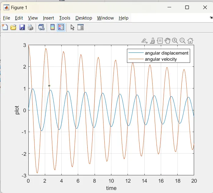
PLOT:
ANIMATION VIDEO :https://youtu.be/wDCN-KRnScE
RESULTS: As can be seen from the above graph and animation video, it is evident that due to low damping coefficient the motion is more and it is continuous. An increase in damping coefficient increases the resistance for the motion.
CONCLUSION: ODE45 simulates high order differential equations efficiently