Week 4.1 - Solving second order ODEs
Logic of Code:
We start off the code with 'clear all', 'close all', and 'clc'.
> Key in all the constant variables with the values.
> Give the initial conditions of the problem.
> This problem requires a time constrain (t_span), which uses a function (linspace()) to get the values of time from 0-20 seconds with 500 intervals for good resolution.
> We call in the ode45() function from which we have defined as below. This function recieves values of time,angle,b,g,l and m.
> We assign a name for the array of variables which have to be stored ([t,results]). The data will be stored in the array called 'results'.
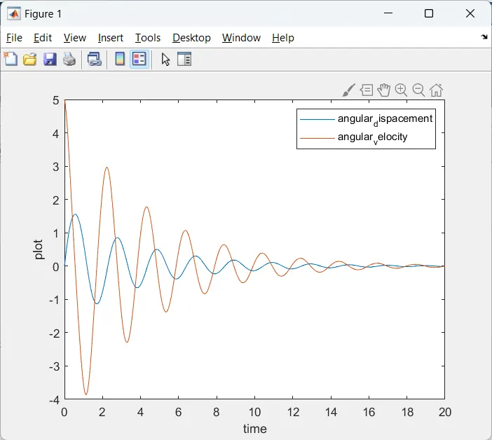
> Now we plot the graph of angular velocity and angular displacement in a plot vs time graph. The values for which will be stored in the array 'results'.
> We use the 'legend()' function to label the respective curves.
> Then begins the for loop iteration for creating the animation.
> Before we start the for loop we give the desired part of the 'results' a variable, say in this code 'theta2'.
> ct=1 for the initial frame.
> We assign another variable 'THETA2' in order to help in the iteration with the iteration variable 'i'.
> x0,y0 are the points of the top of the pendulum.
> X1,Y1 are the coordinates with which we need a line to represent the length of the pendulum visially. Their values are w.r.t the x axis with angle 'THETA2'.
> Then we begine the code for the animation of the pendulum.
> We use 'figure(1)' and 'figure(2)' to differenciate the two results.
> We use the pause function with which rate we want the osillation to run.
> The syntax for making the movie is as follows.
movie(M) %plays the movie in matrix 'M' once
videofile = VideoWriter('pendulum.avi','uncompressed AVI'); %assigns a name and format for the video file
open(videofile) %opens the video file
writeVideo(videofile,M) %writes the video in said file
close(videofile) %closes the file
Matlab code:
% solving second order ode using MATLAB

clear all
close all
clc
%inputs

b = 0.05;
g = 9.81;
l = 1;
m = 0.1;

%initial conditions
theta_0 = [0;5];

% time points

t_span = linspace(0,20,500);

% Solving the ode

[t,results] = ode45(@(t,theta) ode_func(t,theta,b,g,l,m),t_span,theta_0);


% plotting
figure(1)

plot(t,results(:,1))
hold on
plot(t,results(:,2))
xlabel('time')
ylabel('plot')
legend('angular_dispacement','angular_velocity')

% for loop iteration
theta2 = results(:,1);
ct = 1;

for i = 1:length(theta2)
    THETA2 = theta2(i)


 x0 = 0;
y0 = 0;

X1 = l*sin(THETA2)
Y1 = -l*cos(THETA2)
% animation code
figure(2)
 plot([-1 1],[0 0],'linewidth',2,'color','b')
 axis([-2 2 -2.5 2.5])
 hold on
 plot(x0,y0,'s','markersize',15,'markerfacecolor','m')
 hold on
 plot([x0 X1],[y0 Y1],'linewidth',7,'color','y')
 plot(X1,Y1,'o','markersize',20,'markerfacecolor','k')
 grid on
 hold off

 pause(0.007)

 M(ct) = getframe(gcf);
 ct = ct+1

end

movie(M)
videofile = VideoWriter('pendulum.avi','uncompressed AVI');
open(videofile)
writeVideo(videofile,M)
close(videofile)
%The code for definition the function

% ode function definition

function [dtheta_dt] = ode_func(t,theta,b,g,l,m)

theta1 = theta(1)
theta2 = theta(2)
dtheta1_dt = theta2;
dtheta2_dt = -(b/m)*theta2 - (g/l)*sin(theta1);
dtheta_dt = [dtheta1_dt; dtheta2_dt];


end
Result: