Project 1 - Parsing NASA thermodynamic data

Code explanation :

• To start off in almost all codes we use clear all, close all and clc.
• Now we have to open the file from which we have to take and read(Parse) the data.
• we assign a file handle f1
• and use the fopen() function to open a particular file in the given file directory.
• to read the first line we use gt = fgetl() function to read the line.
• now we dont need the first line. We are interested in the values of the coefficients in the data.
• There is a certain format which is followed here, so inorder to extract the data we need to execute our functions and codes we have to code accordingly.
• After reading the first line we read the scond line which has the name of our species as given in the data
• gt1 is used to store teh second line and we need to convert that line into numbers so that we can navigate around that line easily.
• Now we are required to split that line to get our data (Global temps)
• we use the strsplit() function to split the strig.
• We define the global temperatures which we may or may not use with the progression of the code.
• Next we are required to skip the next three lines which contain data which is not of relevance for the code.
• we do that by using a simple for loop to skip the 3 lines.
• Next we extract the lines with useful data.
• So, accoding to the distribution of the data we need to get all the numbers properly, so we use the exponential operator(in the data) to navigate through the line.
• With the given data we require all the numbers before 'E' except the spaces and +2,3 digits after 'E'.
• this logic is used and shown below.
• Mainly we conert the whole line into a numerical array then we use strfind() to find the 'E'
• Then we navigate with the handle of each line treating each of the line as an array.
• Now we use all the useful data by using variable (a_n) where n would be the array pointer( to navigate through the array and store the coeff values)
• We have to manually do that 3 times for all the coefficients
• get all values and put it in our formulae.
• we get all the values and then we use a function to calculate the Total Molecular Weight of each element with its name.
• So what we have done to store all the graph figures in the folder is given in the code. We assign a variable to each figure with an iteration variable (k).
• Initially we assign k = 1
• Then for each figure we iterate the original value of k and then repeat the same.
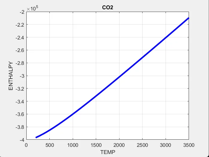
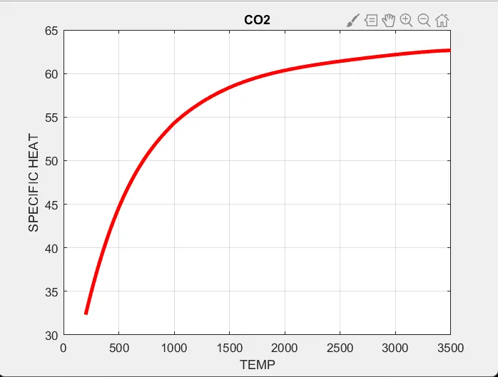
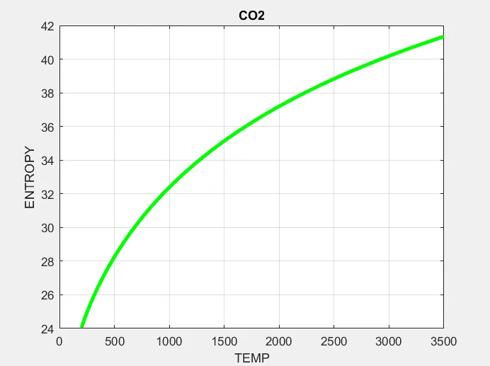
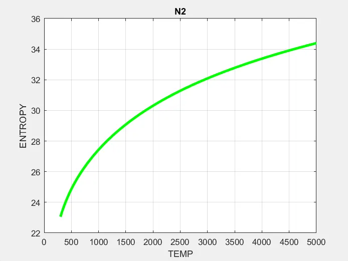
• we plot all the necessary graphs in the 3 different figures.
• The above code will be executed many times and we get 159 images.
• these are stored/saved in a folder using function saveas()
• The results of the same are given below.

Matlab Code:

clear all

close all

clc









% we are going to open the file

f1=fopen('THERMO.dat','r');

gt=fgetl(f1);

% splitting the gt1 to convert it into number

k = 1;

gt1=fgetl(f1);





   

gt1 = strsplit(gt1);

% now converting the cell array into number



global_low_temp=str2double(gt1{2});

global_mid_temp=str2double(gt1{3});

global_high_temp=str2double(gt1{4});



% now skipping the lines which are not having the usefull data

 for l=1:3

     skip_line=fgetl(f1);

 end

   



 for j=1:53

     

% now we need extract the lines from line5 which are having the useful data.



line=fgetl(f1);

% splitting the o string

line_split=strsplit(line);

% converting the cell array into number

atomic_num=str2double(line_split{4});

local_low_temp=str2double(line_split{end-3});

local_high_temp=str2double(line_split{end-2});

local_mid_temp=str2double(line_split{end-1});

%line_num=str2double(line_split{9});

species_name = line_split{1};



% now we need to get the 6th line where we are actually going to calculate

% the coefficients

tline=fgetl(f1);

% we are going to get the locations of the E, so that we can find out the

% coefficients of it.

a=findstr(tline,'E');



% we found the locations of E and with the help of these we can find the

% coefficients,we can get 3 numbers after E using that we can find the

% coeffs. the below 7coefficients are for high temperature.



a1=tline(1:a(1)+3);

a1=str2double(a1);

a2=tline(a(1)+4:a(2)+3);

a2=str2double(a2);

a3=tline(a(2)+4:a(3)+3);

a3=str2double(a3);

a4=tline(a(3)+4:a(4)+3);

a4=str2double(a4);

a5=tline(a(4)+4:a(5)+3);

a5=str2double(a5);



% another 2 coefficients are present in the next line.

tline_2=fgetl(f1);



b=findstr(tline_2,'E');



a6=tline_2(1:b(1)+3);

a6=str2double(a6);

a7=tline_2(b(1)+4:b(2)+3);

a7=str2double(a7);





% the below 7 coefficients are for low temperatures



a8=tline_2(b(2)+4:b(3)+3);

a8=str2double(a8);

a9=tline_2(b(3)+4:b(4)+3);

a9=str2double(a9);

a10=tline_2(b(4)+4:b(5)+3);

a10=str2double(a10);



% the below 4 coefficients are in the next line.



tline_3=fgetl(f1);



c=findstr(tline_3,'E');



a11=tline_3(1:c(1)+3);

a11=str2double(a11);

a12=tline_3(c(1)+4:c(2)+3);

a12=str2double(a12);

a13=tline_3(c(2)+4:c(3)+3);

a13=str2double(a13);

a14=tline_3(c(3)+4:c(4)+3);

a14=str2double(a14);





% assuming the temperature values from low to high global temperature as

% 1000

%  taking the value for universal gas constant.

R=8.314;



 T=linspace(local_low_temp,local_high_temp,1000);



 

%  calculating the specific heat,enthalpy,entropy

 for i=1:length(T)

     

     if T(i)>local_mid_temp

         

       cp(i)=(a1+a2.*T(i)+a3.*T(i)^2+a4.*T(i)^3+a5.*T(i)^4).*R;

       H(i)=(a1+a2.*(T(i)./2)+a3.*(T(i)^2./3)+a4.*(T(i)^3./4)+a5.*(T(i)^4./5)+a6./T(i)).*R.*T(i);

       S(i)=(a1*log(T(i))+a2.*T(i)+a3.*(T(i)^2./2)+a4.*(T(i)^3./3)+a5.*(T(i)^4./4)+a7);

         

     

 

     else

       cp(i)=(a8+a9.*T(i)+a10.*T(i)^2+a11.*T(i)^3+a12.*T(i)^4).*R;

       H(i)=(a8+a9.*(T(i)./2)+a10.*(T(i)^2./3)+a11.*(T(i)^3./4)+a12.*(T(i)^4./5)+a13./T(i)).*R.*T(i);

       S(i)=(a8*log(T(i))+a9.*T(i)+a10.*(T(i)^2./2)+a11.*(T(i)^3./3)+a12.*(T(i)^4./4)+a14);

         

   

     

     end

 end



 

 mkdir('E:\praneeth\programs',species_name);

 

 

 p1 = figure(k);



plot(T,cp,'linewidth',3,'color','r')

grid on

title(species_name)

xlabel('TEMP')

ylabel('SPECIFIC HEAT')





p2 = figure(k+1);



plot(T,H,'linewidth',3,'color','b')

grid on

title(species_name)

xlabel('TEMP')

ylabel('ENTHALPY')



p3 = figure(k+2);

plot(T,S,'linewidth',3,'color','g')

grid on

title(species_name)

xlabel('TEMP')

ylabel('ENTROPY')



k = k+3;



path1 =sprintf('E:/praneeth/programs/%s/temp_vs_cp.png', species_name);

path2 =sprintf('E:/praneeth/programs/%s/temp_vs_H.png', species_name) ;

path3 =sprintf('E:/praneeth/programs/%s/temp_vs_S.png', species_name);



saveas(p1,path1)

saveas(p2,path2)

saveas(p3,path3)



% calculating the molecular weight of each species





disp(species_name)

Total_mol_wt=molecular_weight(species_name);





 



 

 end

 

 function total_m_wt=molecular_weight(species_name)





 element={'O','C','H','Ar','N','S'};

 

 Atomic_mass=[15.999,12.011,1.008,39.948,14.007,32.06];

 

total_m_wt=zeros(1,length(species_name));

 

 for i=1:length(species_name)

     

     if isnan(str2double(species_name(i)))

         

         for j=1:length(element)

             if strcmp(species_name(i),element(j))

             total_m_wt(i)=total_m_wt(i)+Atomic_mass(j);

             end

         end

     else

        total_m_wt(i-1)=total_m_wt(i-1)* str2double(species_name(i));

         

     end

 end

             

   

           total_m_wt=sum(total_m_wt)



end

Results:

Molecular weights in the command window

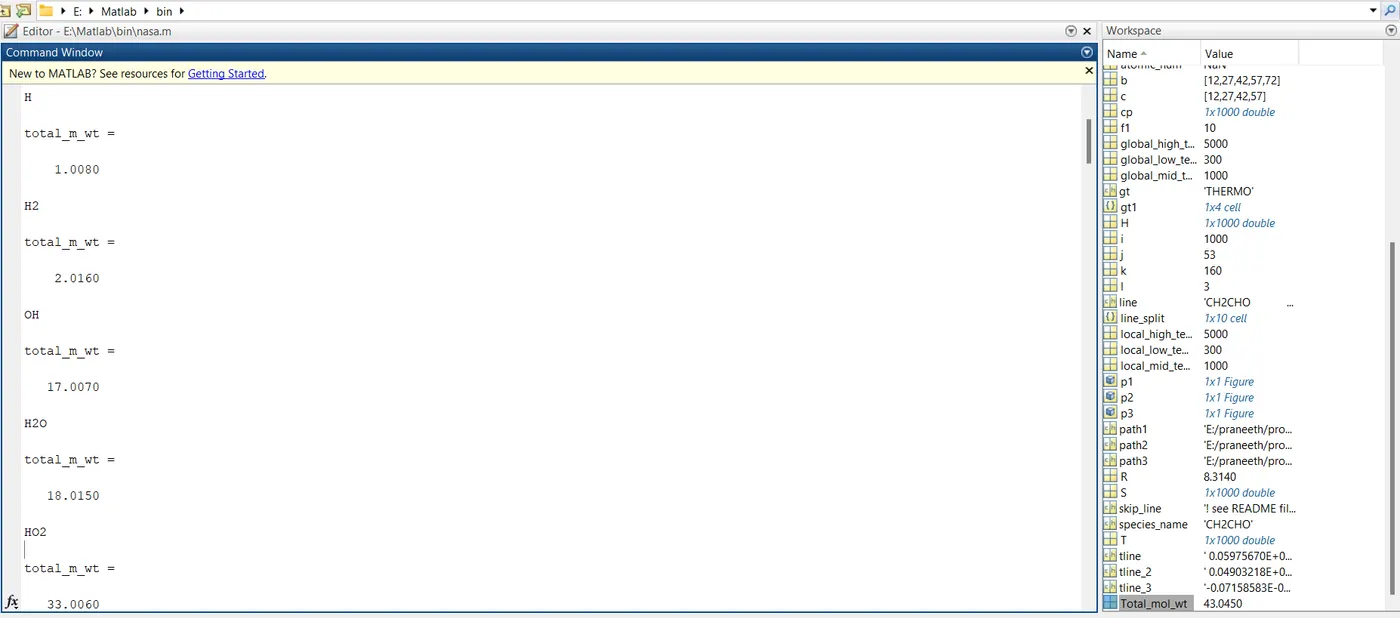
all the files are saved in the assigned directory

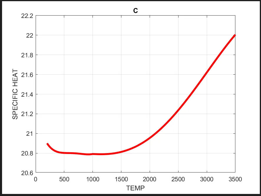
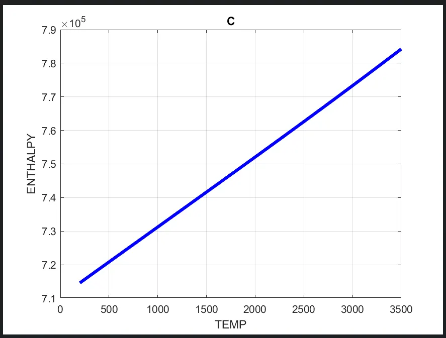
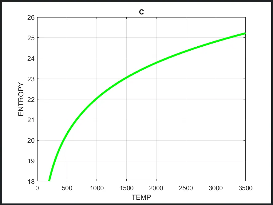
Example plots of carbon C:

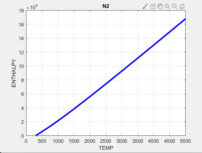
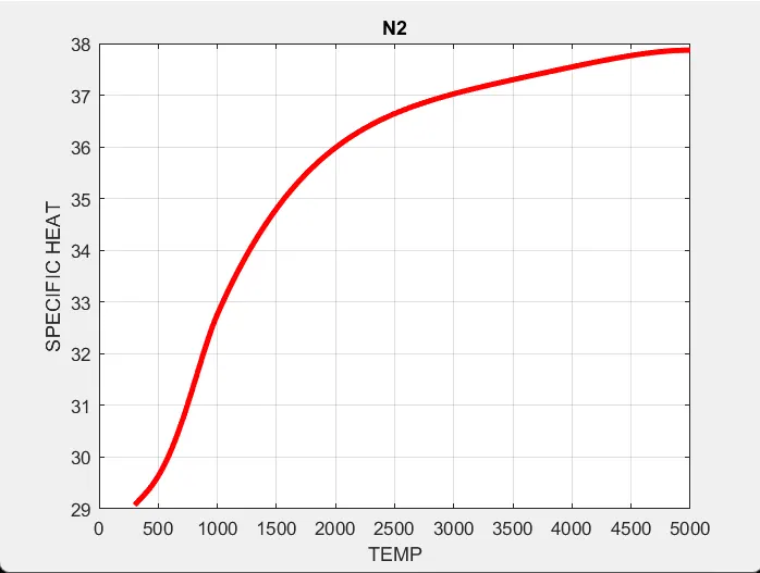
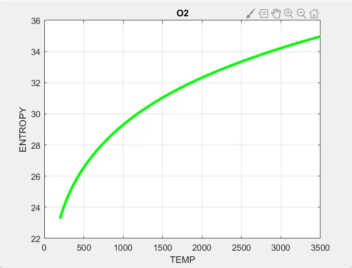
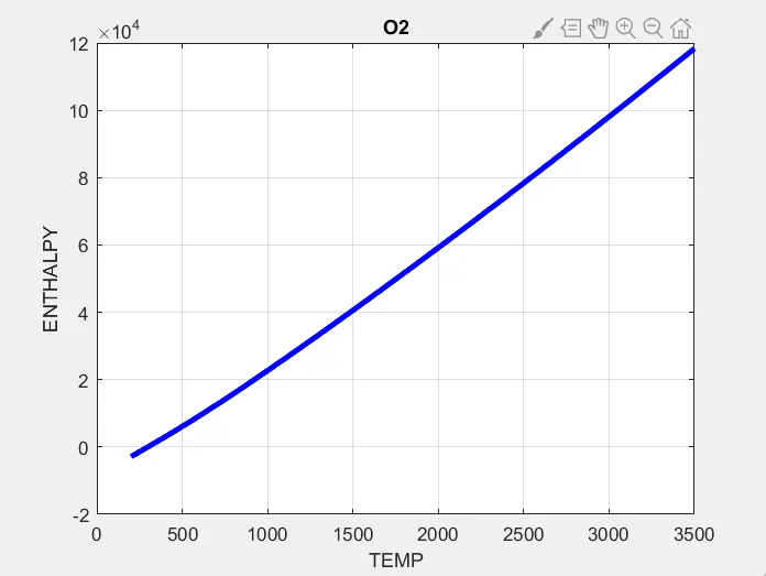
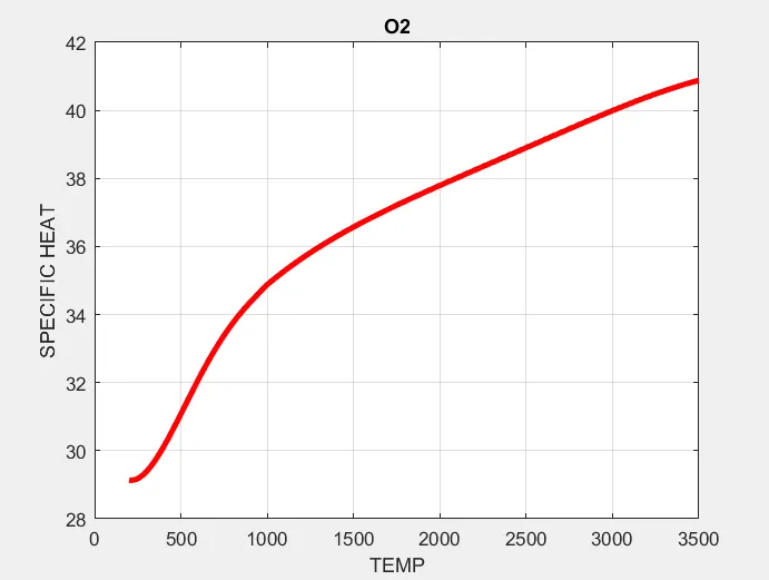
the plots of O2,N2,Co2 are attached below

error:

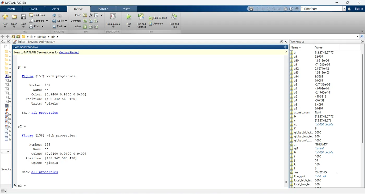
p1,p2,p3 are displayed and semicolon was missing.

Also when running mkdir() with no name change the mkdir() command shows as already exists.