Project 2 - Rankine cycle Simulator

Coding logic:

• We start off the code with the basic clear functions. clear all, close all and clc.
• Now to input the values that we need in real time we use a slightly different approach in writing this code.
• Initially, we use the fprintf() command to display whatever we want, in this case, it is our stages of working of a Rankine cycle engine.
• Now we use the input() command to input the variables which we want during the execution of the code and assign a handle for the same.( P1, T1,T2).
• Then we use the XSteam () in built library function which we downloaded from this challenge to fetch the data of the enthalpy, entropy and saturated temperatures.
• The function XSteam is a defined function which acts like a steam table which we used to use in college for turbomachine calculations.( steam and water)
• we do the same with the following syntax
• H1 = XSteam('h_pt',P1,T1) % ENTHALPY
  S1 = XSteam('s_pt',P1,T1) % ENTROPY
  Hf1 = XSteam('hL_p',P1) % ENTHALPY OF SATURATED LIQUID
  Hg1 = XSteam('hV_p',P1) % ENTHALPY OF SATURATED VAPOUR
  Ts1 = XSteam('Tsat_p',P1) % SATURATED TEMPERATURE
  Sf1 = XSteam('sL_p',P1) % ENTROPY OF SATURATED LIQUID
  Sg1 = XSteam('sV_p',P1) % ENTROPY OF SATURATED VAPOUR

• here, h_pt is for fetching the enthalpy values at pressure P1 and Temp T1.
• s_pt = entropy values at P1 and T1.
• hL_p = enthalpy values at liquid state at pressure P1.
• hV_p = enthalpy values at vapour state at pressure P1.
• Tsat_p = Saturated temp at pressure P1.
• sL_p = Entropy of the saturated liquid at P1.
• sV_p = Entropy of saturated vapour at P1.

• We do this for all the state points accordingly.
• That is we have equations to find all the other required points.
• after we're done with fetching the data values from the XSteam () library function, we use those to proceed with the calculations
• Now that we have our values we can start plotting the T-S and the H-S graphs using the plot() command.
• I have taken the critical temperature as 400-degree celsius
• we now assign a variable t for the critical temp and create an equal space array for the same with the linspace command.
• This is for helping us with the iteration that is useful for the plotting of the saturation curve.
• After plotting the saturation curve we move on to plotting the cycle curve.
• In the case that if x (dryness fraction)>1, we plot the graphs, if this fails we have another plot command for plotting a different kind of cycle.
• We used linspace again to get equally spaced numbers between the two temperatures T1 and T2.
• after plotting the T-S graph we do the same for plotting the H-S graph.
• Now we give all labelling commands to make the plot look better.
• After plotting we move on to do the calculations
• Namely :

1. Turbine work
2. Pump work
3. Heat Addition
4. Heat Rejection
5. Net work done
6. Thermal Efficiency
7. Specific Steam Consumption
8. Back work ratio.

• After the calculations are done, we move on to displaying all the required data that we calculated for future reference
• This is done by using a simple fprinf command for each state point.

% Code to show the t-s and H-s diagram of the Rankine 


clear all
close all
clc


% displaying the information
fprintf('RANKINE CYCLE')
fprintf('\n 1-2 ISENTROPIC EXPANSION')
fprintf('\n 2-3 CONSTANT PRESSURE HEAT REJECTION')
fprintf('\n 3-4 ISENTROPIC COMPRESSION')
fprintf('\n 4-5 CONSTANT PRESSURE HEAT ADDITION')

% Now we write a code to accept inputs in real-time

P1 = input('\n Input the Pressure at turbine inlet (in bar): ');
T1 = input('\n input the temperature at turbine inlet(in degree celcius): ');
P2 = input('\n Enter the pressure at the turbine outlet(in bar): ');;


% At state point 1 

H1 = XSteam('h_pt',P1,T1) % ENTHALPY
S1 = XSteam('s_pt',P1,T1) % ENTROPY
Hf1 = XSteam('hL_p',P1)   % ENTHALPY OF SATURATED LIQUID
Hg1 = XSteam('hV_p',P1)   % ENTHALPY OF SATURATED VAPOUR
Ts1 = XSteam('Tsat_p',P1)  % SATURATED TEMPERATURE
Sf1 = XSteam('sL_p',P1)   % ENTROPY OF SATURATED LIQUID
Sg1 = XSteam('sV_p',P1)   % ENTROPY OF SATURATED VAPOUR

% At state point 2

S2 = S1;
Sf2 = XSteam('sL_p',P2);
Sg2 = XSteam('sV_p',P2);

x = (S2-Sf2)/(Sg2-Sf2);   % DRYNESS FRACTION

Hf2 = XSteam('hL_p',P2);
Hg2 = XSteam('hV_p',P2);

H2 = Hf2+ x*(Hg2-Hf2);

T2 = XSteam('T_ph',P2,H2);
Ts2 = XSteam('Tsat_p',P2);

% At state point 3

H3 = Hf2;
S3 = Sf2;
T3 = T2;
P3 = P2;


% At state point 4

P4 = P1;
S4 = S3;
H4 = XSteam('h_ps',P4,S4);
T4 = XSteam('T_ps',P4,S4);


t = linspace(0,400,500) % Temp


% T-S DIAGRAM plotting

figure(1)
hold on

% saturation curve
 

for i = 1:length(t)
    STL(i) = XSteam('sL_T',t(i))
    STV(i) = XSteam('sV_T',t(i))
   
end
plot(STL,t,'.','color','b')
   plot(STV,t,'.','color','b')
 
% Cycle plot

plot([S1 S2],[T1 T2],'linewidth',1,'color','r')
if x>1
    T3 = Ts2;
    plot([S2 Sg2 S3 S4],[T1 Ts2 T3 T4],'linewidth',1,'color','r')
    T2 = Ts2;
else
    plot([S2 S3 S4],[T2 T3 T4],'linewidth',1,'color','r')
    
end

l = linspace(T1,T2,1000);

for i = 1:length(l)
    plot(XSteam('s_pT',P1,l(i)),l(i),'.','color','r')
end
legend('SAT CURVE')


plot([Sf1 Sg1],[Ts1 Ts1],'linewidth',2,'color','r','DisplayName','cycle plot')
xlabel('ENTROPY [KJ/KG-K] ')
ylabel(' TEMP [K] ')
title('T-S Diagram ')
xlim([0 10]);
ylim([0 500]);


% H-S Diagram Plotting

figure(2)
hold on


% saturation curve

for i = 1:length(t)
    plot(XSteam('sL_T',t(i)),XSteam('hL_T',t(i)),'*','color','b')
    plot(XSteam('sV_T',t(i)),XSteam('hV_T',t(i)),'*','color','b')
   
end
legend(' SAT CURVE')

% Cycle plot

plot([S1 S2 S3 S4 S1],[H1 H2 H3 H4 H1],'linewidth',2,'color','k','DisplayName','cycle plot')
xlabel('ENTROPY [KJ/KG-K] ')
ylabel(' ENTHALPY [KJ-KG] ')
title('H-S Diagram')
ylim([0 3600])
xlim([0 12])


% Calculations

% TURBINE WORK (W_t)

W_t = H1-H2;

% PUMP WORK (W_p)

W_p = H4-H3;


% Heat Addition (Q_in)

Q_in = H1-H4;

% Heat rejection (Q_out)

Q_out = H2-H3;


% Net work done (W_net)
W_net = W_t - W_p;

% Thermal efficiency of the turbine (Therm_eff)

Therm_eff = (W_net/Q_in)*100;

% Specific Steam Consumption (SSC)
SSC = (3600/W_net);

% Back Work Ratio (BW_R)
BW_R = (W_p/W_t)







% RESULTS


fprintf('\n\n RESULTS\n')
fprintf('\n AT STATE POINT 1')
fprintf('\n P1 = %f.2 bar\n',P1)
fprintf('\n T1 = %f deg celcius\n',T1)
fprintf('\n H1 = %f KJ/KG\n',H1)
fprintf('\n S1 = %f KJ/KG-K\n',S1)


fprintf('\n\n RESULTS\n')
fprintf('\n AT STATE POINT 2\n')
fprintf('\n P2 = %f.2 bar\n',P2)
fprintf('\n T2 = %f deg celcius\n',T2)
fprintf('\n H2 = %f KJ/KG\n',H2)
fprintf('\n S2 = %f KJ/KG-K\n',S2)


fprintf('\n\n RESULTS\n')
fprintf('\n AT STATE POINT 3\n')
fprintf('\n P3 = %f.2 bar\n',P3)
fprintf('\n T3 = %f deg celcius\n',T3)
fprintf('\n H3 = %f KJ/KG\n',H3)
fprintf('\n S3 = %f KJ/KG-K\n',S3)


fprintf('\n\n RESULTS\n')
fprintf('\n AT STATE POINT 4\n')
fprintf('\n P4 = %f.2 bar\n',P4)
fprintf('\n T4 = %f deg celcius\n',T4)
fprintf('\n H4 = %f KJ/KG\n',H4)
fprintf('\n S4 = %f KJ/KG-K\n',S4)

Result:

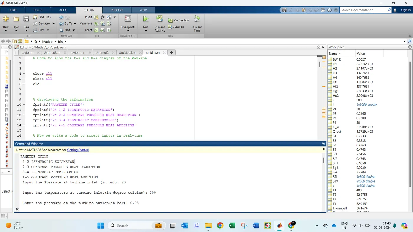
values entered:

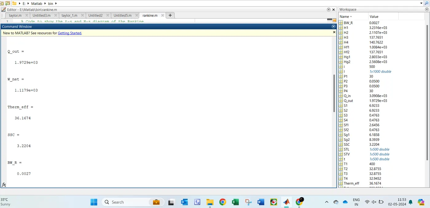
Output of net work output and back work done:

Values of P,T,H and S at point 1,2,3,4

RESULTS

AT STATE POINT 1

P1 = 30.000000.2 bar

T1 = 400.000000 deg celcius

H1 = 3231.571027 KJ/KG

S1 = 6.923259 KJ/KG-K

RESULTS

AT STATE POINT 2

P2 = 0.050000.2 bar

T2 = 32.875490 deg celcius

H2 = 2110.708212 KJ/KG

S2 = 6.923259 KJ/KG-K

RESULTS

AT STATE POINT 3

P3 = 0.050000.2 bar

T3 = 32.875490 deg celcius

H3 = 137.765119 KJ/KG

S3 = 0.476254 KJ/KG-K

RESULTS

AT STATE POINT 4

P4 = 30.000000.2 bar

T4 = 32.945189 deg celcius

H4 = 140.762226 KJ/KG

S4 = 0.476254 KJ/KG-K

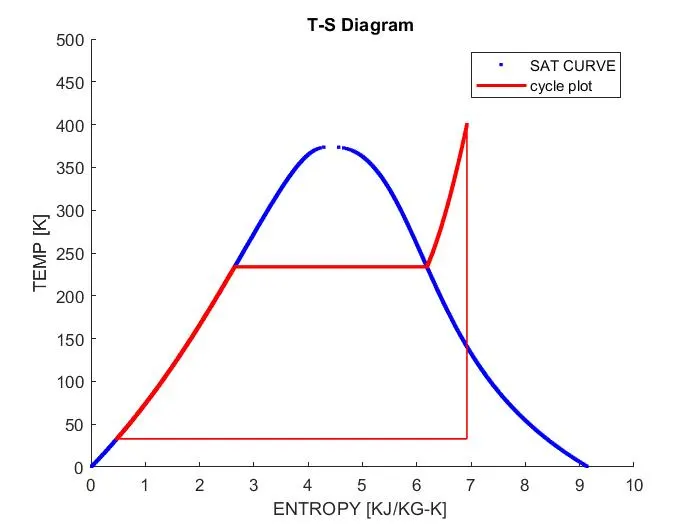
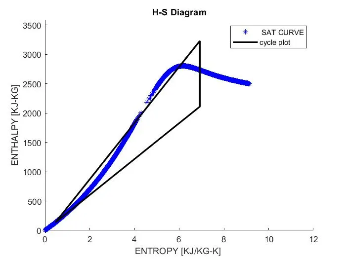
Plot of the Rankine cycle:

T-S Plot:

H-S diagram:

Errors:

kept different brackets for entropy when stating the xlabel so the Matlab program could not interpret it and gave an error

corrected it by debugging.