Week 4.1 - Solving second order ODEs

Week 4.1 - Solving second order ODEs:

AIM:

• To solve the 2nd order ode equation and create animation of the pendulum with given parameters.

Introduction to Second order ode equation:

• In engineering aspects differential second order equation is relation between Acceleration,Angular velocity and displacement.
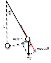
• Let take the simple pendulum as given below,

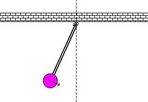
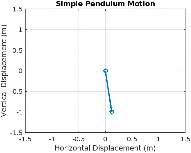
• In this challenge they need animation video in avi formate,for that we have to code as per logic.
• Given below equation is second order ode equation,here t is time,g is gravity,L is length of the pendulum,m is mass,b is damping coefficient.

Given question:

Write a program in Matlab\Octave that will simulate the pendulum motion, just like the one shown in the start of this challenge.

use,

L=1 metre,

m=1 kg,

b=0.05.

g=9.81 m/s2.

Simulate the motion between 0-20 sec, for angular displacement=0,angular velocity=3 rad/sec at time t=0.

Solution:

• From above question we had some parameters like,
  • L=1 metre,
  • m=1 kg,
  • b=0.05.
  • g=9.81 m/s2
  • and t = 0 to 20 sec,
  • Displacement = 0
  • angular velocity = 3 rad/sec
• So now we need to create psuedocode for programming,

Psuedocode and explaination for programming:

• Asusual we start with close all,clear all and clc
• Then give the input like
• b = 0.05; //damping coefficient
• g = 9.81; //gravity
• l=1; //length
• m=1; //mass
• At the initial condition the displacement was 0 and angular velocity is 3,so for that we have to create the column vector like,
  • theta_0 =[0;3];
• Then we need to create line for Time points that,here we create the t_span array that starts from 0 to 20 sec with 500 points,using linspace command.
  • t_span = linspace (0,20,500);
• Then we need to create line for ODE that,here t is time array and we get results as a column vector.
• Then here ode45 is inbuild ode solver in matlab,
• Now we need to define the function as @(t,theta) for time and theta value,
• Next we need to use the function that 'ode_func',
• It is a predefine fuction that contains the value of input parameters
  • [t,results] = ode45(@(t,theta) ode_func(t,theta,b,g,l,m),t_span,theta_0);
  • function dydt = ode_func(~, theta, b, g, l, ~)
    % ODEs for a simple pendulum
    dydt = zeros(2, 1);
    % First ODE: d(theta)/dt = omega
    dydt(1) = theta(2);
    % Second ODE: d(omega)/dt = -b*omega - (g/l)*sin(theta)
    dydt(2) = -b * theta(2) - (g / l) * sin(theta(1));
    end

• In this function we have the ode equations for to find the angles that theta 1 and theta 2.
• Then comming to the plotting,we need to create plotting in column vector methode like
  • figure(1)
    plot(t,results(:,1))
    hold on
    plot(t,results(:,2))
• Then we need to create xlabel,ylabel,legend and title as like below.
  • ylabel ('Plot')
    xlabel('Time')
    legend('Location', 'best');
    title('Solving 2nd order equation')

• Then comming to the animation setup
• Plot empty lines for Angular Displacement and Angular Velocity Set labels and title for the plot
• Then Create Figure 3 Plot empty line for Simple Pendulum Animation Set axis limits, labels, and title for the animation plot Preallocate video file 'pendulum_animation.avi'
• Next Open the VideoWriter object with the specified filename For each time step in t Calculate pendulum bob coordinates (x, y) based on results(i, 1)
• Then Update animation plot with the new coordinates Force MATLAB to update the figure (drawnow)
• And Capture the current frame for the video Write the frame to the video file Pause for a short duration
• Finally Close the video file Set labels and title for the animation plot in Figure 3.

MATLAB CODE:

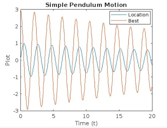
OUTPUT PLOT:

AVI Screen shot:

ANIMATION GOOGLE DRIVE LINK:

https://drive.google.com/file/d/1C5MPbwetbFBESn4pyJFCg_RCeBA7GS-2/view?usp=sharing

https://drive.google.com/file/d/1npYu0F5JneSah5lSrUJZ_949as4FNVKD/view?usp=sharing

Conclusion:

• From this Challenge I learned about Second order ode equation in MATLAB.