Week 4.1 - Solving second order ODEs

This ODE represents the equation of motion of a simple pendulum with damping.

Here,

let's assume 'theta' to be 'theta1', convert the 2nd order ODE to 1st order, so-

assuming, d(theta1)/dt = theta2;

d(theta2)/dt + b*theta2/m + g*sin(theta1)/L=0

=> d(theta2)/dt = -b*theta2/m - g*sin(theta1)/L

%Main Code

%Solving second order ODEs of pendulum
clear all
close all
clc

% inputes
L=1;       % length of the pendulum in m
m=1;       % mass of the ball in kg
b=0.05;    % damping coefficient
g=9.81;    % gravity in m/s^2

%intial angular displacement and velocity of the pendulum
theta_i=[0;3]; %given 3 rad/s and converted to m/s

%time period
tp=linspace(0,20,500);

%ODE
[t,rst] = ode45(@(t,theta) odef(t,theta,b,g,L,m),tp,theta_i);

%plotting

figure(1)
plot(t,rst(:,1));     % Plot angular displacement vs time
hold on
plot(t,rst(:,2));     % Plot angular velocity vs time
pause(0.03);
xlabel('Time');
ylabel('Plot');

% Create a figure for the animation
figure(2)
x = L * sin(rst(:, 1));    % Compute x-coordinate based on the angular displacement
y = -L * cos(rst(:, 1));   % Compute y-coordinate based on the angular displacement
ct=1;                      % Counter variable declaration
for i = 1:length(t)

    plot([0, x(i)], [0, y(i)], 'LineWidth', 2);             % Plot the line representing the pendulum
    hold on
    plot(0,0,'*','color','g');                              % Plot the pendulum pin
    plot(x(i), y(i), '*', 'MarkerSize', 20, 'Color', 'r');  % Plot the pendulum bob
    hold off
    axis([-L-1, L+1, -L-1, 2]);                           % Set the axes limits
    title('Animated Pendulum');                           % Set the title of the plot
    pause(0.03);                                          % Pause for a short duration for smooth animation
    movi(ct)=getframe(gcf);                               % Capture the current frame
    ct=ct+1;

end

%movie creation
movie(movi)                                                % Display the animation as a movie
videofile=VideoWriter('ODE_Pendulum.avi','Uncompressed AVI');   % Create a video file
open(videofile)                                            % Open the video file for writing
writeVideo(videofile,movi)                                 % Write the frames to the video file
close(videofile)  

#ode function creation

function [dtheta_dt] = odef(t,theta,b,g,L,m)

  theta_1=theta(1);
  theta_2=theta(2);
  dtheta1_dt = theta_2;
  dtheta2_dt = -(b.*theta_2)/m - (g.*sin(theta_1))/L;
  dtheta_dt = [dtheta1_dt; dtheta2_dt];

end

Explanation:

main code

1. The code is solving the second-order ordinary differential equations (ODEs) that describe the motion of a pendulum.
2. The input parameters for the pendulum system are defined: the length of the pendulum (L), mass of the ball (m), damping coefficient (b), and gravitational acceleration (g).
3. The initial angular displacement and angular velocity of the pendulum are set. Here, the initial displacement is 0 radians, and the initial velocity is 3 radians per second.
4. A time vector tp is created using the linspace function. It ranges from 0 to 20 seconds and contains 500 equally spaced points.
5. The ODEs are solved using the ode45 function, which numerically integrates the equations over the time vector tp. The results are stored in t (time) and rst (angular displacement and velocity).
6. A figure is created, and the angular displacement and angular velocity are plotted as functions of time.
7. Another figure is created for the animation of the pendulum.
8. Inside the animation loop, the position of the pendulum is calculated based on the angular displacement using trigonometric functions.
9. The line representing the pendulum is plotted from the pivot point to the current position.
10. The pendulum pin (pivot point) is plotted at coordinates (0, 0).
11. The pendulum bob is plotted at the current position.
12. The axes limits are set to ensure the pendulum is visible in the plot.
13. The title of the plot is set to "Animated Pendulum".
14. A short pause is added to achieve a smooth animation.
15. The current frame of the figure is captured using the getframe function and stored in the movi array.
16. The counter variable ct is incremented after each frame.
17. After the animation loop, the captured frames are displayed as a movie using the movie function.
18. A video file named 'ODE_Pendulum.avi' is created using the VideoWriter function.
19. The captured frames are written to the video file using the writeVideo function.
20. The video file is closed.

function code

1. Defines the ODE function odef that describes the dynamics of the pendulum.
2. The function takes inputs t (time), theta (angular displacement and velocity), and the system parameters (b, g, L, m).
3. It computes the derivatives dtheta1_dt and dtheta2_dt based on the current values of theta and the system parameters.
4. The derivatives are returned as a column vector dtheta_dt.
5. This function is used by the ode45 solver to numerically integrate the ODEs.

Errors faces

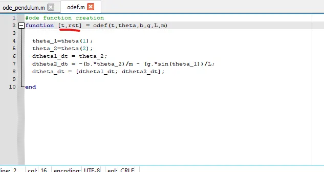
Here since I have written t,rst so the graph was showing 2 parabolas. Then i found the mistake and rectified to 'dtheta_dt'.

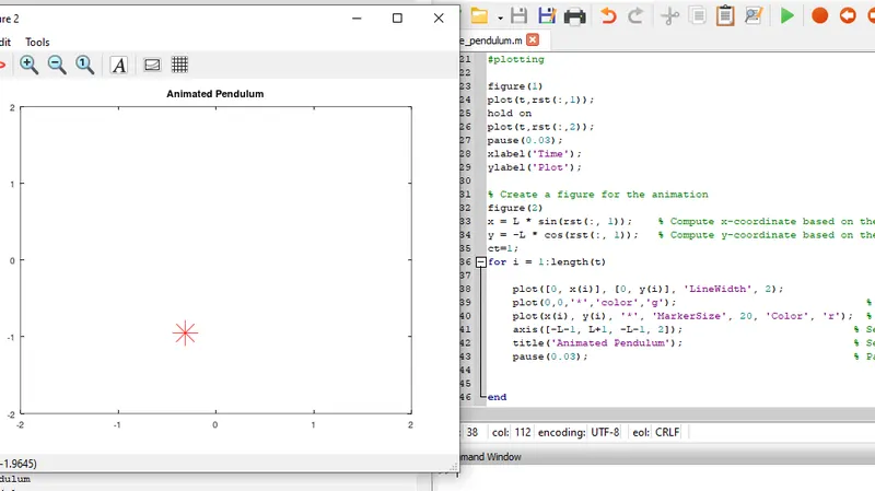
Here, since I have not used the 'hold on' function after plotting the pendulum bar, so it was not shoeing it. So I rectified it and place the 'hold on' and now it is rectified.

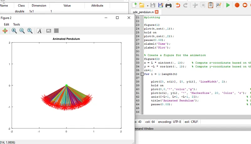
Here, since I have not used hold off, so it is continually holding each an every iteration of the pendulum. so i placed a hold off after the pendulum bob plot.

Video link: https://youtu.be/6uh1QIGmRdw