Week 4.1 - Solving second order ODEs

Aim: -

To Solve the ODE which represents the equation of motion of simple pendulum with damping.

Objectives:-

To write a program that solve the following ODE which represents the equation of motion of simple pendulum with damping and create an animation vidoe of output by solving this ODE.

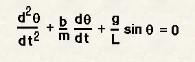
Theory:

The motion of a simple pendulum is a basic classical example of simple harmonic motion, consisting of small bob and a massless string. Movemnet of the pendulum depends on Newton's second law. When this law is written, a second order ordinary differential equation is formed that describe the position of the end pendulum w.r.t time.

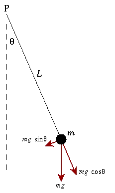
• g = gravity in m/s^2.
• L = Length of the pendulum in meter.
• m = mass of the ball in.
• Damping coefficient.

Since the given function is in seconfd order differential equation we will convert it into first order to solve the ODE

Let

θ=θ1 

                dθ1/dt=θ2

                dθ^2/dt^2=dθ2/dt

Input

• L = 1 meter
• m = 1 kg
• b = 0.05
• g = 9.81 m/s^2
• Time span = 0-20 sec
• Angular displacement = 0.
• Angular velocity = 3 rad/sec^2 at time t = 0

Code:-

clear all
close all
clc

b = 0.05;     % Damping Coefficient
g = 9.81;     % Acceleration due to gravity
l = 1;        % Length of string
m = 0.1;      % Mass of the bob
ct = 1;       % Counter variable

% Initial condition

theta_0 = [0;5];      % Displacement at an angle

% Time points 

t_span = linspace(0,10,500);

% Solve ODE

[t, output] = ode45(@(t, theta) ode_func(t, theta, b, g, l, m), t_span, theta_0);


figure(1)
hold on
plot(t, output(:,1))
plot(t, output(:,2))
ylabel('x-axis')
xlabel('y-axis')
grid on


theta2 = output(:,1);
for i = 1:length(theta2);

    theta_x = theta2(i);

    x0 = 0;
    y0 = 0;

    x1 = l*sin(theta_x);
    y1 = -l*cos(theta_x);

    % plotting the pendulum
    figure(2)
    plot([-0.5 0.5], [0 0], 'color', 'b', 'linewidth', 5);
    hold on
    plot([x0 x1], [y0 y1], 'color', 'r', 'linewidth', 2)
    hold on
    plot(x1, y1, 'o', 'markers', 15, 'markerfacecolor', 'y')
    hold off
    grid on
    axis([-1.5 1.5 -1.5 0.5]);
    pause(0.002)
    M(ct) = getframe(gcf);
    ct = ct+1;
end

movie(M)
videofile = VideoWriter('pendulum.avi', 'Uncompressed AVI')
open(videofile)
writeVideo(videofile,M)
close(videofile)

Function Code:-

function [dtheta_dt] = ode_func(t, theta, b, g, l, m)

theta1 = theta(1);
theta2 = theta(2);

dtheta1_dt = theta2
dtheta2_dt = -(b/m)*theta2 - (g/l)*sin(theta1) 

dtheta_dt = [dtheta1_dt; dtheta2_dt];

end

Detail explanation each step of the program.

1. In the first step input and initial condition of simple pendulum are fed.

2 Then the program is written to solve the ODE in which MATLAB inbuit function (ode45) is used with constant theta, t, and another function is used, which is defined seperately in function program.

3. In the nest step result of solved ODE is plotted w.r.t time using plot command.

4. Now iteration of co-ordinate is fed using for loop to creat animation.

5. Then plot command is used to plot pendulum string and bob

6. In the next step, the move command is used to creat an animation video oscillating pendulum.

Output:

The output obtained is graphical representation velocity curve and displacement curve w.r.t time

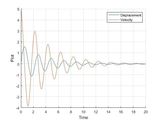
Errors: No major errors were thrown in the command window while coding.

Link:

https://youtu.be/uQE3QoAHNg0