Project 1 - Parsing NASA thermodynamic data

Aim:-

To  write a code in MATLAB to parse nasa thermodyanmic data file and then calculate thermodyanamic properties of various gas species

Objective:-

write a function that extracts the 14 coefficients and calculate the specific heat, enthalpy and entropy for all the species in the data file.

Calculating molecular weight of each species.

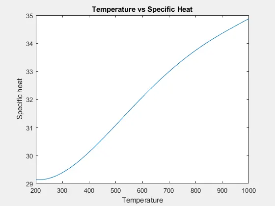
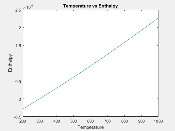
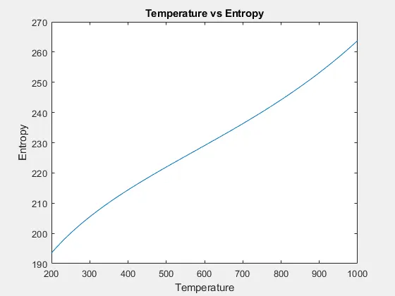
Plotting the specific heat, enthalpy and entropy for the local temperature range.

saving the plots as images with appropriate names and dumping them in seperate folder for each species.

Theory:-

File parsing:

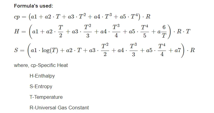
File parsing refers to examining a file. Using file parsing, data can be extracted from the file which can be stored and be used to perform calculations. Here a thermodynamic file generated by NASA is parsed from which the high temperature and low temperature of various species are extracted and further stored to calculate the Specific heat (c_p), Enthalpy(H) and Entropy(S)

Specific heat(c_p):

Specific heat is defined as the heat required to raise the temperature of a given mass by a unit temperature. It is denoted by 'Cp'. Its unit is J/K.

Enthalpy:

Enthalpy refers to the internal energy of a system which includes the temperature and pressure in an enclosed system, the change in heat is refered to as Enthalpy of the system. It is denoted as 'H'. Its unit is J/K.

Entropy(S):

Entropy is a function of state of a system. It is an extenal property and is reversible. Entropy plays and important part in thermodnyamics is based on entropy which says that entropy of an isolated system never decreased. It is denoted as 'S'. Its unit is J/K.

From the program point of view

It can be seen that 1st line is the title and the 3rd, 4th and 5th lines are just comments,  Which are not in scope of parsing(they don't possess any value data for our calculations) 

The 2nd line has 3 temperature value which are the global temperature for the entire data set. This can be stored in a variable and also not significant for our calculation as each species in particular to plot and calculate. 

From the 6th line the species data start and goes up to the end of the dataset.  It can easily be noted a significant pattern in the species data distribution. 

That is each species has 4 lines of data. 

1st species line has,  the local low,  high and mid temperature respectively. 

Whereas the 2nd to 4th species line has the 14 coefficient values. 

The first 7 coefficient are high temp coefficient,  i.e the temperature value above mid temperature must be used in order to calculate Cp,  H and S. and other 7 coefficient are low temp coefficient.

 

Program:

% File parsing

clear all
close all
clc

% Reading data from the file 
f1=fopen('THERMO.dat','r')

% Reading header information
fgetl(f1);

% Global temperature
t_line=fgetl(f1);
a=strsplit(t_line,' ');

% Extracting the global temperature range
global_low_temp=str2double(a{2});
global_mid_temp=str2double(a{3});
global_high_temp=str2double(a{4});

% Neglecting the 3 lines
fgetl(f1);
fgetl(f1);
fgetl(f1);

% Reading species block
% Line1
for i=1:53
    t_line2=fgetl(f1);
    s=strsplit(t_line2,' ');
    species_name=s{1};
    A=strfind(t_line2,'G');
    temp_values=t_line2(A+4:length(t_line2));
    B=strsplit(temp_values,' ');

    local_low_temp=str2double(B{1});
    local_mid_temp=str2double(B{2});
    local_high_temp=str2double(B{3});

t_line=fgetl(f1);
b=findstr(t_line,'E')

% 1st coefficient
b1=t_line(1:b(1)+3);
b1=str2num(b1);

%2nd coefficient
b2=t_line(b(1)+4:b(2)+3);
b2=str2num(b2);

%3rd coefficient
b3=t_line(b(2)+4:b(3)+3);
b3=str2num(b3);

%4th coefficient
b4=t_line(b(3)+4:b(4)+3);
b4=str2num(b4);

%5th coefficient
b5=t_line(b(4)+4:b(5)+3);
b5=str2num(b5);

%Line 2
line2=fgetl(f1);

%6th coefficient
b6=line2(1:b(1)+3);
b6=str2num(b6);

%7th coefficient
b7=line2(b(1)+4:b(2)+3);
b7=str2num(b7);

%8th coefficient
b8=line2(b(2)+4:b(3)+3);
b8=str2num(b8);

%9th coefficient
b9=line2(b(3)+4:b(4)+3);
b9=str2num(b9);

%10th coefficient
b10=line2(b(4)+4:b(5)+3);
b10=str2num(b10);

%Line 3
line3=fgetl(f1);

%11th coefficient
b11=line3(1:b(1)+3);
b11=str2num(b11);

%12th coefficient
b12=line3(b(1)+4:b(2)+3);
b12=str2num(b12);

%13th coefficient
b13=line3(b(2)+4:b(3)+3);
b13=str2num(b13);

%14th coefficient
b14=line3(b(3)+4:b(4)+3);
b14=str2num(b14);

% Universal gas constant
R=8.314;

t=linspace(local_low_temp,local_high_temp,100);

% To calculate
% Specific heat by creating function
c_p=specific_heat(b1 ,b2 ,b3 ,b4 ,b5, b8 ,b9 ,b10 ,b11 ,b12 ,local_mid_temp ,t ,R);

% Enthalpy by creating function
H=enthalpy(b1 ,b2 ,b3 ,b4 ,b5 ,b6 ,b8 ,b9 ,b10 ,b11 ,b12 ,b13 ,local_mid_temp ,t ,R);

% Entropy by creating function
S=entropy(b1 ,b2 ,b3 ,b4 ,b5 ,b7 ,b8 ,b9 ,b10 ,b11 ,b12 ,b14 ,local_mid_temp ,t ,R);

% Creating folder
mkdir(['F:\MATLAB\',species_name]);
cd(species_name);


% Plotting for

% Temperature vs Specific heat
figure(1)
plot(t,c_p)
xlabel('Temperature')
ylabel('Specific heat')
title('Temperature vs Specific Heat')
image=getframe(gcf);
imwrite(image.cdata,'T vs C_p.png')
saveas(1,'Specific Heat','jpg')

% Temperature vs Enthalpy
figure(2)
plot(t,H)
xlabel('Temperature')
ylabel('Enthalpy')
title('Temperature vs Enthalpy')
image=getframe(gcf);
imwrite(image.cdata,'T vs H.png')
saveas(2,'Enthalpy','jpg')

% Temperature vs Entropy
figure(3)
plot(t,S)
xlabel('Temperature')
ylabel('Entropy')
title('Temperature vs Entropy')
image=getframe(gcf);
imwrite(image.cdata,'T vs S.png')
saveas(3,'Entropy','jpg')

cd ..

% Calculating molecualr mass
M=molecular_wt(species_name);
K=sprintf('%s mol_wt=%f',species_name,M);
disp(K)
end

Fuction for Specific heat

% Function for Specific Heat

function c_p=specific_heat(b1 ,b2 ,b3 ,b4 ,b5, b8 ,b9 ,b10 ,b11 ,b12 ,local_mid_temp ,t ,R)

if (t>local_mid_temp)

    c_p=(b1+(b2.*t)+(b3.*(t.^2))+(b4.*(t.^3))+(b5.*(t.^4)))*R;

else
    c_p=(b8+(b9.*t)+(b10.*(t.^2))+(b11.*(t.^3))+(b12.*(t.^4)))*R;

end

Function for Enthalpy

% Function For Enthalpy

function H=enthalpy(b1 ,b2 ,b3 ,b4 ,b5 ,b6 ,b8 ,b9 ,b10 ,b11 ,b12 ,b13 ,local_mid_temp ,t ,R)

if (t>local_mid_temp)

    H=(b1+((b2.*t)/2)+((b3.*(t.^2))/3)+((b4.*(t.^3))/4)+((b5.*(t.^4))/5)+(b6./t)).*t*R;

else

    H=(b8+((b9.*t)/2)+((b10.*(t.^2))/3)+((b11.*(t.^3))/4)+((b12.*(t.^4))/5)+(b13./t)).*t*R;

end

Function for Entropy

% Function For Entropy

function S=entropy(b1 ,b2 ,b3 ,b4 ,b5 ,b7 ,b8 ,b9 ,b10 ,b11 ,b12 ,b14 ,local_mid_temp ,t ,R)

if (t>local_mid_temp)

    S=((b1.*log(t))+(b2.*t)+((b3.*(t.^2))/2)+((b4.*(t.^3))/3)+(b5.*(t.^4))+b7)*R;

else

   S=((b8.*log(t))+(b9.*t)+((b10.*(t.^2))/2)+((b11.*(t.^3))/3)+(b12.*(t.^4))+b14)*R;

end

Function for Molecular weight

% Function for molecular weight

function M=molecular_wt(species_name)

atomic_mass=[15.999, 1.008, 12.011, 14.007, 39.948];
elements=['O', 'H', 'C', 'N', 'A'];

mol_wt=0;
for i=1:length(species_name)
    for j=1:length(elements)
        if strcmpi(species_name(i),elements(j))
            mol_wt=mol_wt+atomic_mass(j);
            z=j;
        end
    end
    t=str2double(species_name(i))
    if (t>1)
        mol_wt=mol_wt+(atomic_mass(z)*(t-1));
    end
end
M=mol_wt
end

Explanation

1) The program is Commerced with the basic 'clear all',  'close all',  'clc' commands. 

2) f1=fopen(THERMO.dat, ' ') 

In order to open the file,  the 'fopen command is used,  'THERMO. dat' is the file name and 'r' related to reading the file.  This is saved as a variable of f1 for further reference. 

3) fgetl(f1)

    t_line=fgelt(f1) 

    a=strsplit(t_line, ' ') 

From this step,  the process of line reading is started.  The 'fgetl' command is used for this purpose. The variable that was saved is now used for reading the line from that .dat file.

Dividing the file into a pattern of 4 lines,  i.e 1st line contains species name and local temperature and rest three contains coefficient. 

4) fgetl(f1) 

    fgetl(f1) 

    fgetl(f1) 

Use to neglect first three lines. 

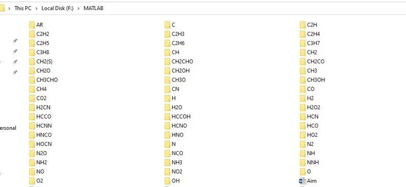
5)There are totally 53 species as explained below,

Total lines = 218

Irrelevant lines  = 6

Total relevant species lines = 218-6 =212

So,  number of species = 212/4=53 species. 

For i=53

t_line2=fgetl(f1);

s=strsplit(t_line2,' ');

species_name=s{1};

A=strfind(t_line2, 'G');

temp_value=t_line2(A+4: length(t_line2));

B=strsplit(temp_values, ' ');

Using a 'for' loop with the 53 species  and with fgetl command each line of species is read and the coefficient values are stored from b1 to b14. 

Line number two consist of the global Temperature range. For extracting the values we use the split tactic, where we identify a delimiter that acts as a reference point.  We initiate this by using the 'strsplit' command. For our case ' ' (literally space mark) is the delimiter where either side is the space hosts the temperature value. Since we can identify on which position the values lie with respect to space. 

t_line=fgetl(f1);

b=findstr(t_line, 'E');

The string values are concerted to number characters using 'str2num'

6)  value of universal gas constant we know, 

R = 8.314

7) Used seperate function for 'specific heat',  'Enthalpy' and 'Entropy'

8) 'Molecular_wt' function used to calculate the molecular weight. 

9) Now the extracted data is saved in a directory with the species name using the 'mkdir' command. cd cammaand is used for changing the current directory. 

10) Basic plot command are further given for comparison between all three thermodynamics properties and the temperature range.  All plots are saved to directory using saved as command. 

The directory is converted back to the current one and the master loop is finally ended. The . dat file is also closed.

Explaination for

Function of Soecific Heat, Enthalpy and Entropy

 1) Since the coefficient available in data file is having a temperature constant, an if condition is used.

2) First 7 coefficients are high temperature coefficent and last 7 are low temperature coefficient, to calculate the thermodynamic property vlues , coefficient are selected reference to temperature range.

Explaination for

Function of molecular weight

1)A character array is defined for the atoms and of atomic weights respectively to character array is defined.

2)The input string is compared with the character array, when a match occurs associated atomic weight is taken.

3)For molecular having number defining the number of atoms, the number i first extracted oand calculation is made to account for multiple atomic weights.

4) A variable is assigned to store the output value of the function.

Output :

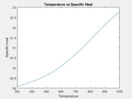
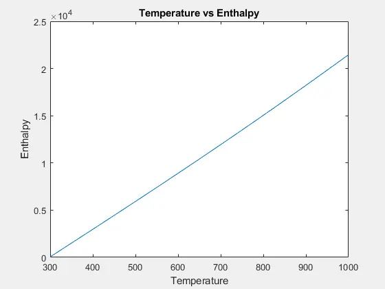
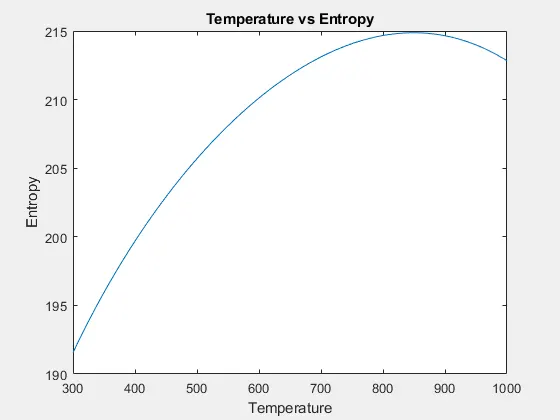
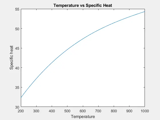
Some random output plots and molecular weight calculation:

 For O2

For N2

 For CO2

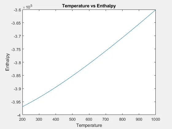
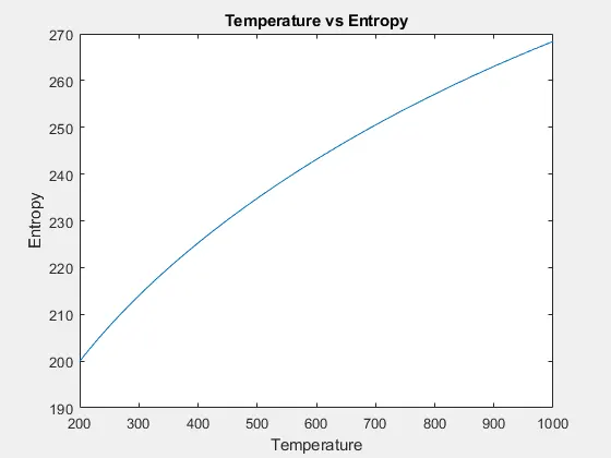
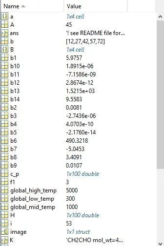
Output values of workspace

53 Files

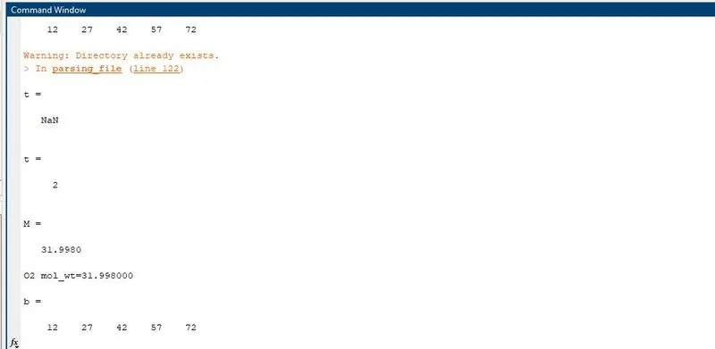
Molecular weight

Conclusion:

On successful parsing of data from NASA thermodynamic data file, variation of thermodynamic properties with temperatur of ceritain species of molecular are observed with the help of plots obtained.