Week 4.1 - Solving second order ODEs

Aim: To solve a simple pendulum's second-order ordinary differential equation and animation of the damping effect.

Objective:

1. Using the built-in MATLAB function for solving ordinary differential equations to create the function.

2. To create a simple pendulum animation.

Code explanation:

1) The given data from the problem statement represent the code's initial inputs. Where the input of the time domain for the entire code will run is then created. The command linspace is used to define the time in seconds from 0 to 30 and a value of 100 in between.

2) For calculating angular displacement and velocity equation of motion is used to plot for given values.

3) Function command is used in the main code to solve the 2nd order equation. other function in the main code computes the array of the time and displacement data.

4)After calculation plotting is done, Then, after saving the movie, we created a for loop for which we are creating the frame motion for the straightforward pendulum.

code:

clear all
close all
clc

%damping coefficient
b = 0.05; 
%acceleration due to gravity  
g = 9.81;
%length of Pendulum in meters   
l = 1;
%mass      
m = 1;       


%inital conditions
%angular displacement & velocity
y_ad_v = [0;5];

%time points for simulation
t_s = linspace(0,30,100);

%solve ode
a = @(t,y) ode_func(y,b,g,l,m);
[t, y] = ode45(a,t_s,y_ad_v);

%Plot of angular displacement & velocity.
figure(1);
hold on

plot(t,y(:,1),'-.','markersize',5,'linewidth',1.5,'markerfacecolor','g');
plot(t,y(:,2),'-.','markersize',2,'linewidth',1.5,'markerfacecolor','k');
title('Angular velocity&Displacement Vs Time')
legend('Angular Displacement','Angular Velocity')
xlabel('Time in seconds');
ylabel('Angular velocity&Displacement');

% animation for pendulum motion

amp = y(:,1);
ct=1;
for i = 1:length(amp)
    G = amp(i);
    x0 = 0;
    y0 = 0;
    %polar co-ordinate to cartesian co-ordinate
    x1 = l*sin(G);
    y1 = -l*cos(G);
    
    figure(2)
    plot([-2 2], [0 0], 'linewidth', 5, 'color', 'b')
    hold on
    plot([x0 x1],[y0 y1],[x1 x1], [y1 y1],'o','markersize',20, 'markerfacecolor', 'r')
    hold off
    axis([-1.5 1.5 -1.5 1.5])
    title(['Time: ', num2str(t_s(i))]);
    pause(0.03)
    M(ct) = getframe(gcf);
    ct= ct+1;

end   

% saving the animation in file directory  
movie(M)
videofile = VideoWriter('Simple Pendulum.avi');
open(videofile)
writeVideo(videofile,M)
close(videofile)

the function in side:

function [dy_dt] = ode_func1(y,b,g,l,m)

y1 = y(1);
y2 = y(2);
dy1_dt = y2;
dy2_dt = -(b/m)*y2 - (g/l)*sin(y1);
dy_dt = [dy1_dt; dy2_dt];
end

Output:

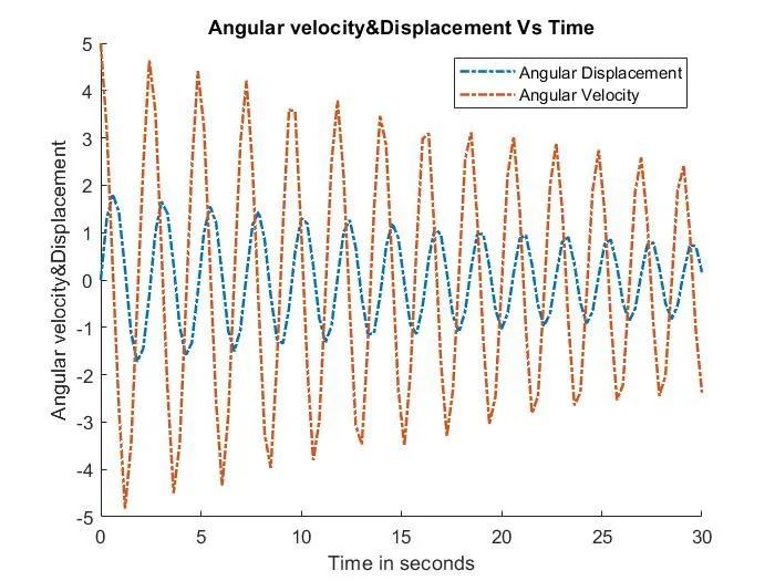
The graph shows that the damping factor causes the displacement to reduce as we advance in time. The plot makes it clear that displacement starts at 0 as the initial condition. The angular velocity vs. time plot shows that it began at 3 rad/sec and has since dropped significantly.

Link to the Animation:

simple pendulum animation

A simple pendulum's second order ordinary differential equation and animating the damping effect.

Conclusion:

Using the MATLAB function ordinary differential equations have been developed.

Hence the simple pendulum animation is shown.