Week 4.1: Project - Steady state simulation of flow over a throttle body

Aim: Steady state simulation of flow over a throttle body

Object:

1. Set up and run the steady-state simulation for flow over the throttle body.
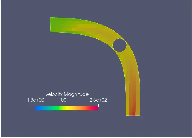
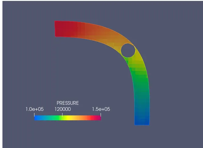
2. Post-process the results and show pressure and velocity contours
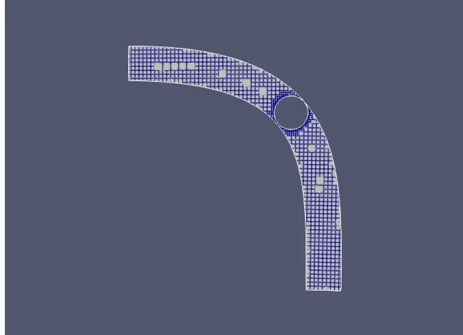
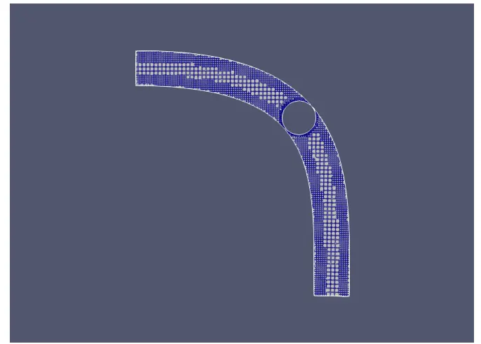
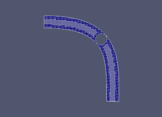
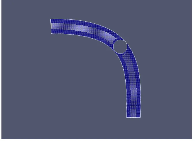
3. Show the mesh
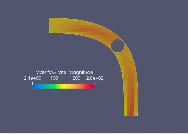
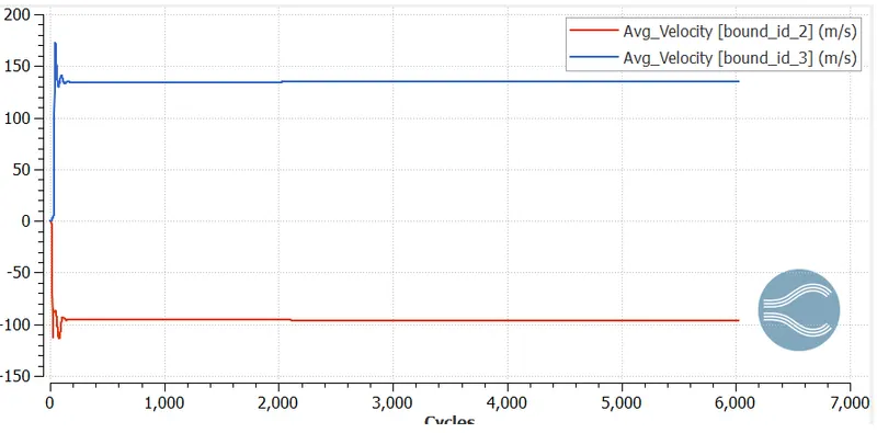
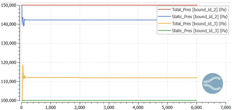
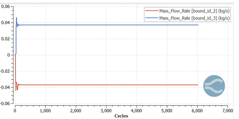
4. Show the plots of pressure, velocity, mass flow rate

Introduction:

A throttle is a mechanism by which the fluid flow is managed by construction or obstruction. An engine’s power can be increased or decreased by the restriction of inlet°, due to the presence of throttle. The term throttle can be used to increase the efficiency of the car, the car accelerator peddal can be used as throttle to increase the efficiency of the engine. It is used as throttle in the field of aviation, known as thrust lever in jet engine powered aircraft for steam locomotive the valve which controls the regulation of gas is called as regulator.

Application of throttle:

The throttle is a mechanism which is used to increase or decrease the power of engine by restricting the flow of inlet gases coming through it there are numerous applications of the throttle mechanism which are listed below

• Internal Combustion Engines
• Fuel Injected Engines
• Reciprocating Engine Aircraft

Case setup:

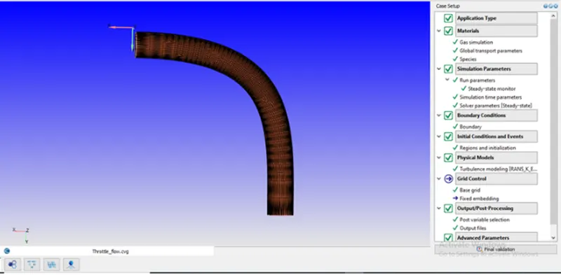
The elbow. STL file is load into the Converge-CFD set-up.

The internal flow simulation does not involve the usage of the external boundary, the external boundary is of special interest when there a OW simulation setup. The external boundary can be deleted by selecting the triangle option from the ribbon and then hitting the button of the keyboard by enabling the hotkeys. The other alternative is selecting the 'Repair' option from the 'Geometry Dock' window and selecting the entity and hitting 'Apply.

The diagnosis dock is select from the Mew' option and the 'Fir, option is select. It is found that there are 211 open edges of the in the geometry (Intersections (0) No manifold Problems (0) Open Edges(211)”overlapping

Base – Grid:

Boundary conditions:

Setting up &Turbulence model:

The Realisable - made! is selected from the case-setup tree for the above-said simulation. Since the size of the eddies is restricted near the wall and the maximum she of the eddies is formed away from the wall. It is well suitable for resolving flows in the logarithmic flow region where y+ ranges from 30th 300 and flows involving a nigh Reynolds number.

Determination of flow velocity:

First of all, let us assume that the flow is incompressible, the Bernoulli Equation for the incompressible flaw states that the sum of the mechanical, potential, and kinetic energy remains constant so any increase in one form may result in

the decrease in another farm. Therefore for the above surface, the equation can be written as

Taking the inlet of the pipe as a reference

Ps + 1/2 ρ v^2 + ρgh = Ptotal

Ps1 = ptotlal - 1/2 ρ v^2 = equation 2

Ps1 + ρ v1^2 / 2 + ρgh + hpump = Ps2 + ρ v2^2 / 2 + ρgh2 + hturbine + HL

Where subscripts 1 & 2 represent the condition at the inlet and the outlet respectively.

The challenge does not mention the pumping head at the inlet, and the turbine head at the outlet respectively. Therefore it can be omitted... pumps however are useful in driving the fluid flow from the inlet to the respective destination by providing the useful head, whereas the turbine is used for extracting the head from the fluid by the turbine.

HL represents the irreversible head loss between inlet and outlet clue to all components of the piping system other.

The total head loss can be equated to the sum of major head loss and the minor head loss

Equation 5

HL_total = HL major + HL minor

HL major = fLv^2 / 2gd

HL minor = K L V1^2 / 2g

Equation 6

HLelbow =Kelbow V1^2 / 2g

Equation 7

HL throttle = Kth throttle V1^2 / 2g

Head loss duo to obstruction in pipe

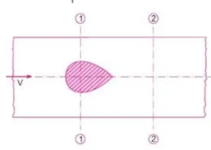
The throttle placed in the direction of fluid flow will act as an obstruction to the flow of fluid

Equation 8

h = (Vc – V)^2 / 2g

Equation 9

The coefficient of contraction =Area of vena contracta / Area of orifice

Ac Vc = Av

Equation 11

Vc = Av / Cc (A – a)

Equation 11

H = V^2 / 2g [ A / Cc (A – a) -1]^2

H = V1^2 / 2g [A / Cc (A – a) -1 ] ^2

The area of throttle is 1.603e – 5m^2

Coefficient of contraction is 0.93066

Coefficient of loss of obstruction is 0.02388

Equation 13

Htotal = (f L/D +0.3+0.4+0.02388)* V1^2 /2g

Length of pipe

1.7339236E -01m

Diameter of pipe

0.0171742m

Friction of pipe is given as

f = 64 / Re

Re = ρ * v * D / u

Equation 13 rewrite as

Htotal = (64 * u / ρ * v * D) L / D +0.3+0.4+0.02388) * V1^2 /2g

Rewrite equation 4 is

Ptotal = Ps2 + ρgh2 + ρV2^2 / 2+((64*u*/ ρ * v*d))L/D +0.3+0.4+0.02388)*V1^2/2G

Equation 14 is

150000 = 100000 + 1.177 * 9.81 *0.119998 +1.77V2^2 / 2+((64 * 1.846e-05/ 1.77*v1*0.017142) 0.177323/ 0.171742 +0.3+0.4+0.02388) * V1^2 /2*g

Calculating Mach number flow:

Mach number is defined as the ratio velocity of the object to the velocity of the sound

Equation 15 written as

M = V/A (or) V/C

M = 282.755/ 346.3

M = 0.816

calculating the density of air inlet using Redlich Kwong equation of state

A cubic equation of state implies an equation that, when expanded, would contain the volume terms raised to the power first second, and third respective! Mon of the common two barometers cubic e notions con be expressed by the equation

Equation 16 is

p= RT/(V-b) - a /T^0.5V(V + b)

a = 0.42748 * R^2 Tc^2.5/Pc

b = 0.08664 * RTc /Pc

R = 287.05 J/kg k

Critical temp Tc = 132.63k

Critical pressure Pc = 3.7858pa

Absolute temp Tc = 300k

a = 1.88626

b = 0.000871281

150000 = 86115/(V-0.000871) - 1.88626 / 17.32V(V + 0.000871)

This is cubic root equation of three values of v

2598000v^3 – 1495111.8v^2 - 1299.19v + 0.00164293

V = 0.57497 – 0.00087

Calculating velocity at the inlet using the following relation for compressible flows:

Equation 17 written as

Pstatic = Ptotal {1 + gama -1/2 * M^2 } ^ (gama – 1/ gama)

Where Mach number M = V/C

C = Root ( gama * R * T)

Rewrite a equation 9 is

Pstatic = Ptotal {1 + gama -1/2 * (V^2 / gama *R*T)} ^ (gama – 1/ gama)

Finally velocity of inlet is 109.54m/sec

HL= 446.07m

Calculating Reynolds number for elbow pipe:

Re = ρ * v * D / u

Where ρ at 300k and 1atm pressure = 1.177 kg / m^3

Dynamic viscosity of the air at 300k is 1.846 e -05kg / m –sec

Calculation the hydrodynamic entrance length Lc for the turbulent flow:

The entrance length in turbulent flow much shorter and dependence on its Reynolds number weaker.

Equation 19

Le = 10*D

Le = 0.171742m

Calculating turbulent boundary layer thickness:

The boundary layer thickness is defined as the thickness at which the viscous velocity becomes 99% of the free stream velocity.

Equation 20 is

del / x = 0.38/Re_x^0.2

del = 0.003970677m

Calculating Skin friction Coefficient

Equation 21

Cf = 0.059 / 979651^0.2

Cf = 0.003589

Calculating Wall Shear, Stress:

Equation 22

Tow_w = 0.5 * ρ * U^2 *Cf

Tow_w = 25.3434N /m

Calculating the frictional velocity:

Equation 23

Ut = Root (Tow_w / ρ)

Ut = 4.6402 m sec^-1

Calculating Reynolds number for the throttle body:

Equation 24

The throttle will act as a flat plate, the characteristics length of the throttle plate will be along the direction of the flow. Therefore Reynolds number or the throttle body is 111817. Since the calculated Reynolds number is less than Rex = 5 * 10^5

Calculating Laminar Boundary Layer Thickness:

The laminar boundary layer thickness for the flat plate

Equation 25 is

Del/x = 4.91 / root (Rex)

Del = 0.000235m

Calculating Skin friction Coefficient tart laminar flat plate:

Equation 26 is

Cflat = 0.664/root(Rex)

Cflat = 0.001985

Calculating Well Shear Stress a laminar flat plate:

Equation 27

Tow_w = 0.5 * ρ * U^2 *Cf

Tow_w = 14.01N /m^2

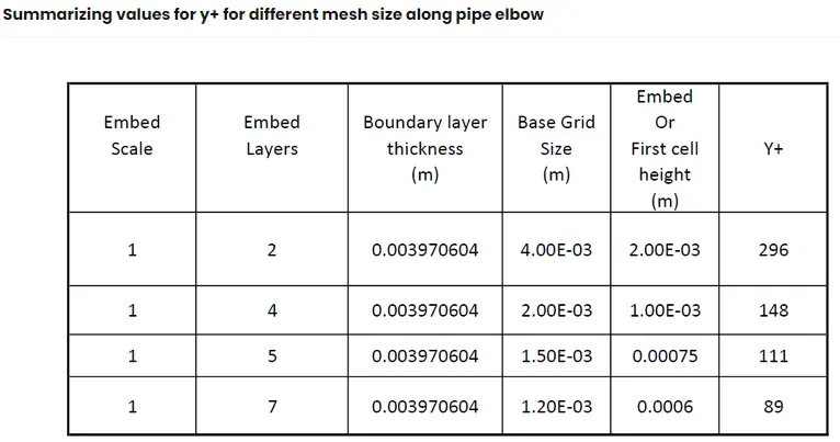
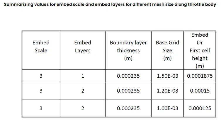
Summarizing all values:

ResultS:

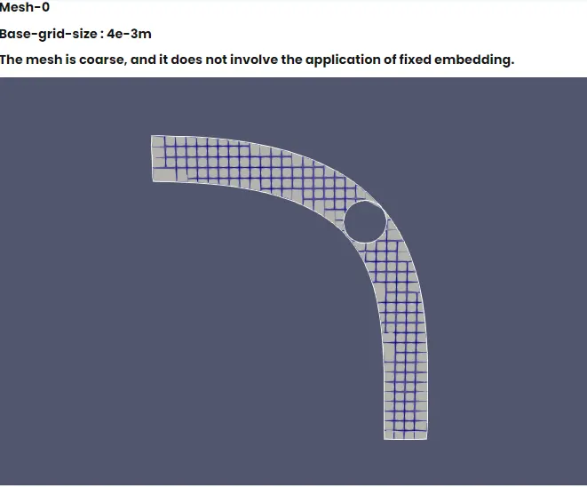
Mesh 1:

Mesh 2:

Mesh 3:

Mesh 4:

Mesh 0

velocity contour plot:

Pressure:

Mass flow rate:

Line plots

Velocity:

Pressure:

Mass flow rate:

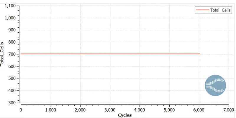
Total cell count: