Week 4.1: Project Steady state simulation of flow over a throttle body

AIM:

To simulate flow over a Throttle Body in a steady-state condition.

INTRODUCTION:

Throttle Body:

In fuel-injected engines, the throttle body is the part of the air intake system that controls the amount of air flowing into the engine, in response to driver accelerator pedal input in the main. The throttle body is usually located between the air filter box and the intake manifold, and it is usually attached to the mass airflow sensor.

PROCEDURE:

A. Geometry Setup:-

• elbow.STL file is imported into converge CFD.
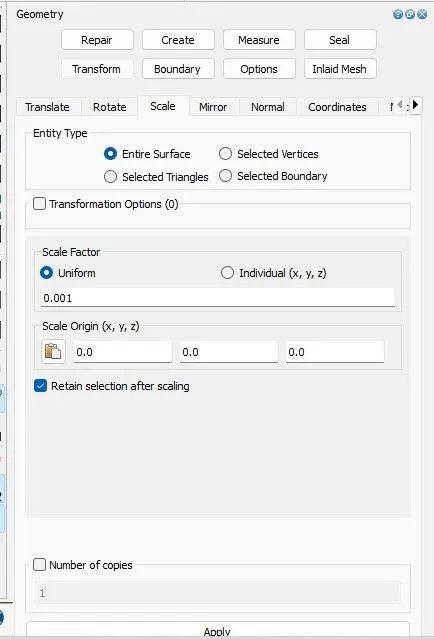
• Geometry is scaled from millimeter to meter.

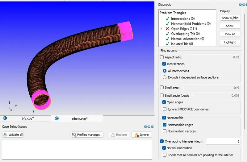
Diagnosis is run to check for any errors:

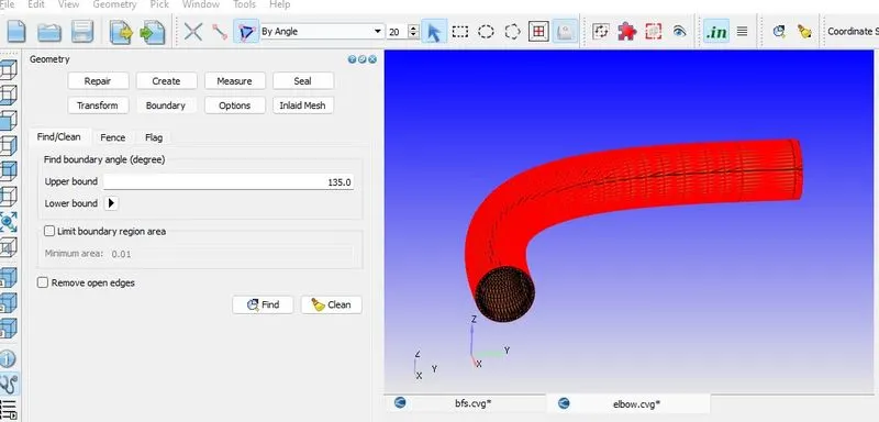
Once we remove the thickness, we will have an open edge. We can use the patch command to close the open edge. To do this, we need to select the edge option and then choose the open edge. After that, we can go to Repair and select Patch to patch the inlet and outlet of the component.

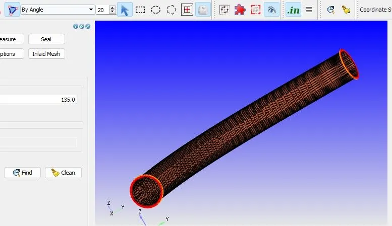
Now, more New Boundaries are flagged as shown below:

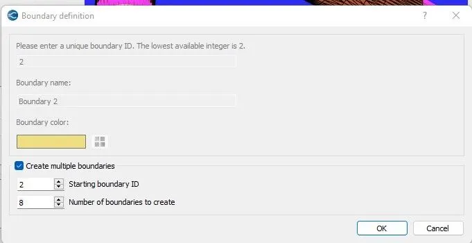
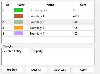
To assign boundaries such as inlet and outlet, we can go to the View option and select Hide Boundaries. Then, we can hide the inlet and outlet boundaries to view the throttle body.

Next, we can click on Diagnosis and select Clear. After that, we can click on the Box Pick option and draw a box around the component to view it in half and see the throttle.

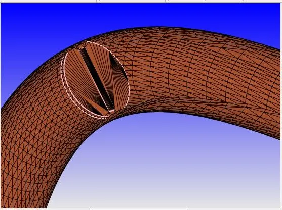
To enable normals, we can click on the Normal option. It's possible that some of the normal points may be outward and some inward, but we can resolve this issue by toggling the Normal option again.

After that, we can click on the Diagnosis option and then select Find to see all the problem triangles that need to be resolved. Once we fix those issues, our boundary flagging will be complete.

We can now proceed to the case setup.

Case Setup:

Application Type: Time-based

Material:

• Air is used as predefined mixtures.
• Gas simulation is enabled
• Reaction mechanism is enabled (mech.dat)

Simulation Parameters:

• Steady State Solver
• Steady-state monitor is enabled.
• Use share memory is checked.

Simulation time parameters:

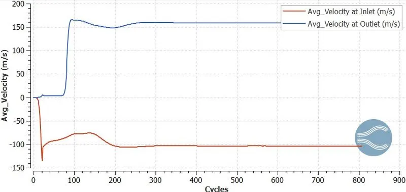
• Average velocity, Total Pressure, and Mass flow rate are monitored at outlet boundary conditions.
• Monitor start delay = 200 cycles
• Sample size = 100 cycles
• Initial time-step = 1e-9
• minimum time-step = 1e-9
• End time = 15000
• Maximum time-step = 1

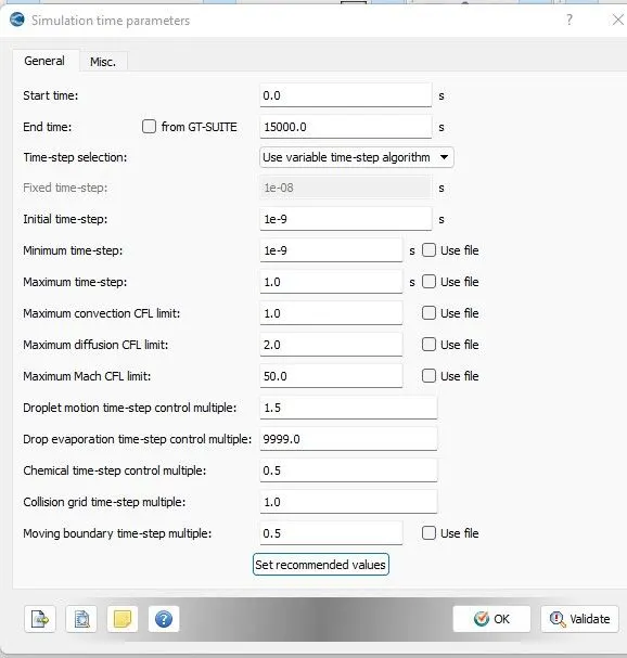
Before moving to the next Assign boundaries

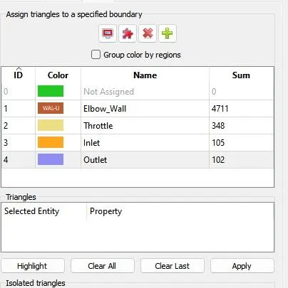
Solver Parameters:

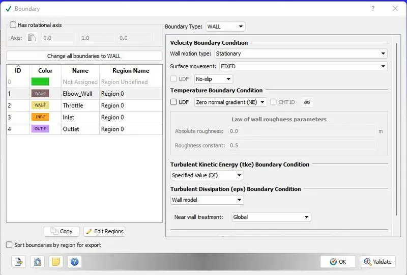
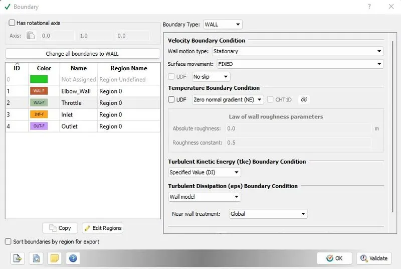
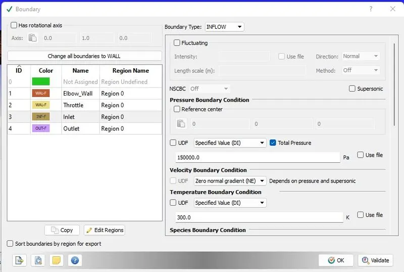
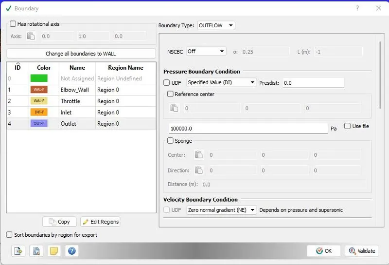
Boundary conditions:-

• Elbow: Wall with No-slip condition.
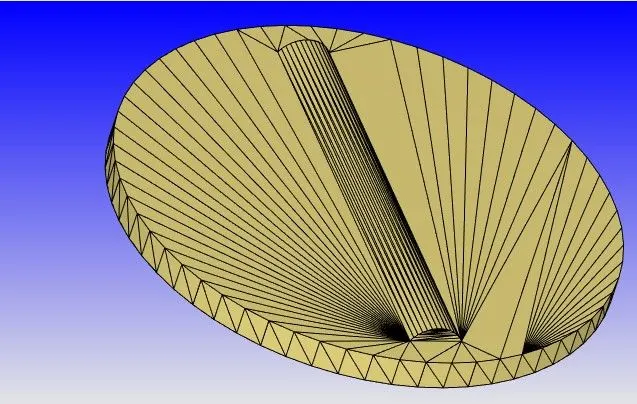
• Throttle Valve: Wall with No-slip condition.
• Inlet: Inflow with Pressure 150000Pa and Air is Added.
• Outlet: Outflow with Pressure 150000Pa and Air is Added.

Region & Initialization:

1. To add a region, namely 'Region 0', first, we need to select all four boundaries from the 'View' option, drag and drop them into 'Region 0', and then click on the OK button.

2. Once the region is added, we need to go to the boundary section and validate it by clicking the right mouse button.

   .

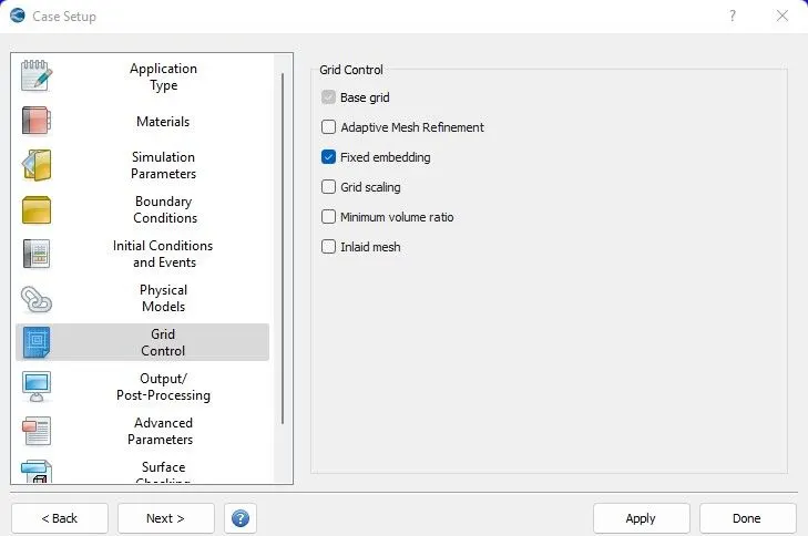
Grid Control:

• Base grid
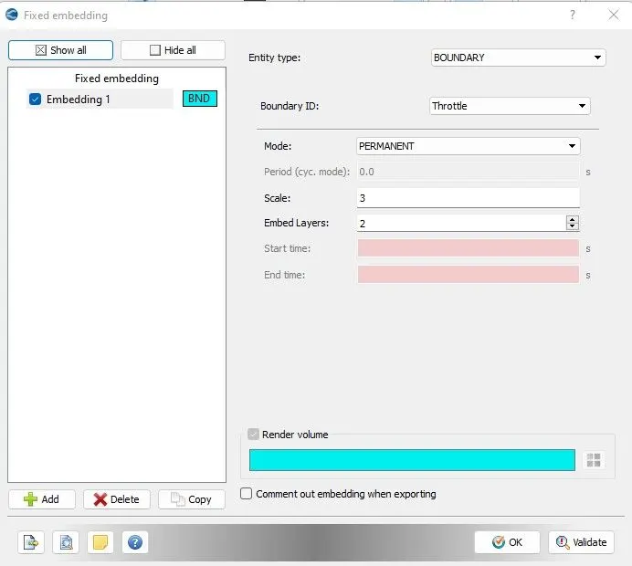
• Fixed Embedding

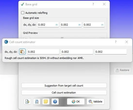
Since the Mesh is not so refined near the throttle, an Embedded System is applied.

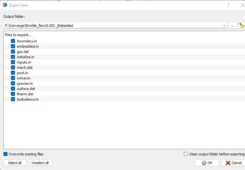
All input files are exported in the directory to simulate Cygwin.

Post-Processing:

• Paraview Results:

1. Mesh:

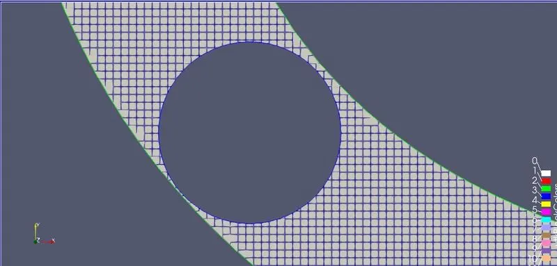
Meshing without Embedding

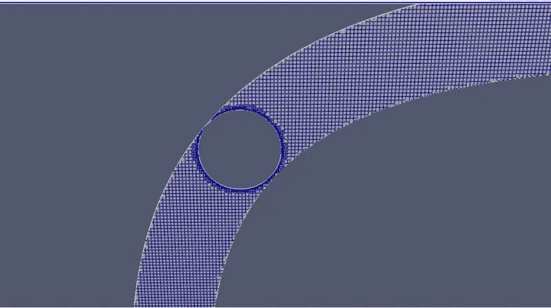
Meshing with Embedding

2. Velocity Contour:

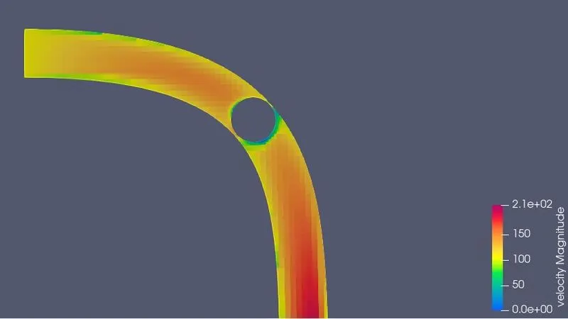
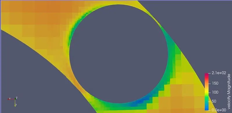
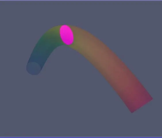
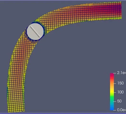
Velocity contour in the throttle valve

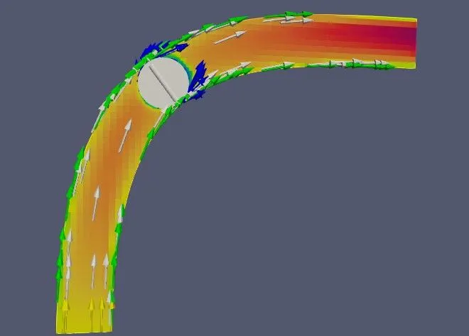
Velocity Contour of fluid flow

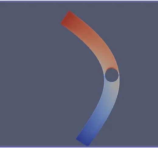
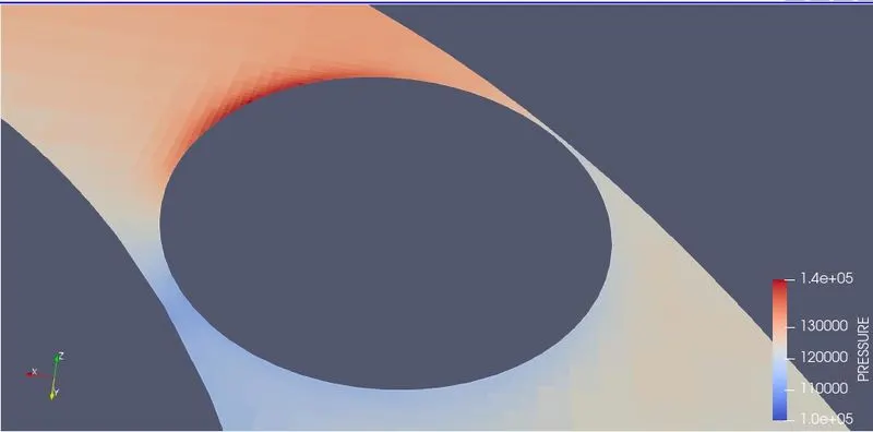
3. Pressure Contour:

4. Throttle Valve:

5. Average Velocity line plot:

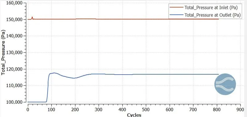
6. Total Pressure line plot:

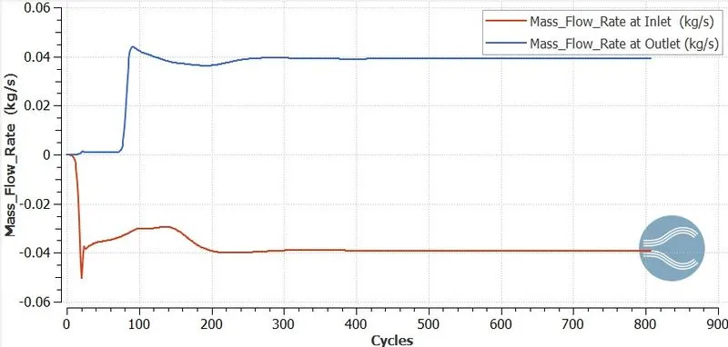
7. Mass Flow Rate line plot:

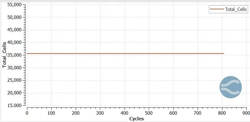
8. Total Cell Count:

ANIMATION:

To create an animation, I will open PARAVIEW and import the file from the destination folder using the .vtm extension. After that, I will click on the Apply button. Next, I will select the slice option and turn off the 'show plane' and 'triangulate the slice' settings. Then, I will set the Z normal icon and click on the Apply button. I will choose the appropriate parameters, such as velocity and pressure, based on the requirements and adjust the color scheme by accessing the color map.

Pressure Animation:

Velocity Animation:

Temperature Animation:

CONCLUSION:

• During a steady-state simulation, the velocity and pressure variables of airflow through the throttle body are observed.
• In a steady-state condition, the throttle valve remains stationary as the airflow passes through the elbow.
• The mass flow rate is measured to be 0.04 kg/s at both the inlet and outlet. Since the throttle valve is stationary and the flow is steady-state, the airflow cannot be controlled.
• There are no changes in cell count throughout the entire cycle.
• High pressure is observed in the inlet of the elbow and the inlet throttle valve region, while high velocity is observed in the outlet of the elbow and the outlet throttle valve region.
• According to Bernoulli's formula, the pressure and velocity are inversely proportional. This means that when pressure increases, velocity decreases while keeping the sum of potential energy, kinetic energy, and pressure constant.