Week 4.1: Project - Steady state simulation of flow over a throttle body

1. Title – Steady state simulation of flow over a throttle body.

2. Objective –

• To create the model of a throttle body in converge Software.
• To set up the case with proper grid size, material and boundary conditions.
• To solve the case using Cygwin terminal and convert the result for Paraview software.
• To import output files in Paraview and generate required contours and plots.

3. Introduction –

Generally, throttle body is tube containing pivoting valve, which is used to regulate the fluid flow in the body. It is mostly used in engines to regulate flow of air mostly, Some, systems use a throttle body with two smaller throats and butterflies instead of one large one. in older carbureted engines, the throttle body is built into the carburetor and via mechanical means and engine vacuum, more fuel is delivered as the valve opens.

Throttle body, itself is associated with many issues like temperature rise, wear and tear etc. so simulation of throttle in throttle body is becomes important, we can find temperature of throttle, mass flow rate with respect to throttle opening, fluid velocity and pressure. In this simulation we are going to simulate flow over throttle body and will generate pressure and velocity contour, which will better insights about throttle functioning.

We performed 2D steady state simulation for flow over throttle body, for that following procedure was followed -

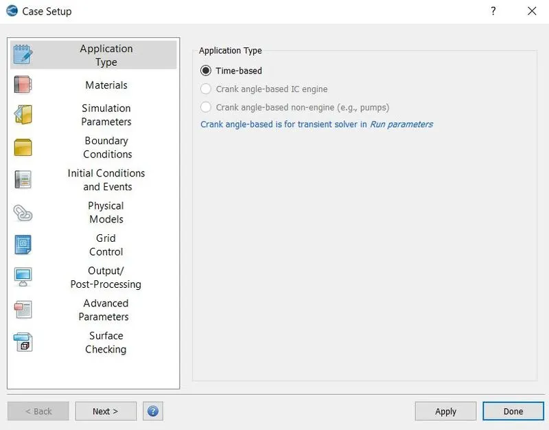
1. Starting with application type, which is time based, since it is not related to IC engine applications.

Case setup- application type

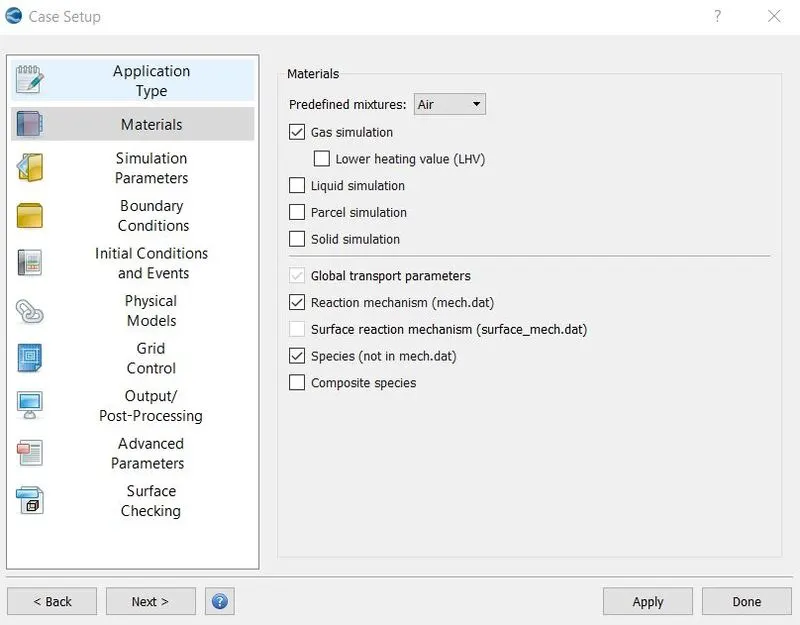
2. Air chosen as fluid material and reaction mechanism was enabled.

Case setup - materials

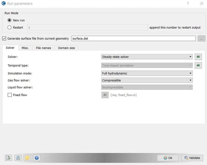
3. In run parameters steady state chosen as solver type, simulation mode was chosen as full hydrodynamic because we want to simulate with effects of fluid also. Enable steady state monitor in miscellaneous menu of run parameter.

Run parameter -

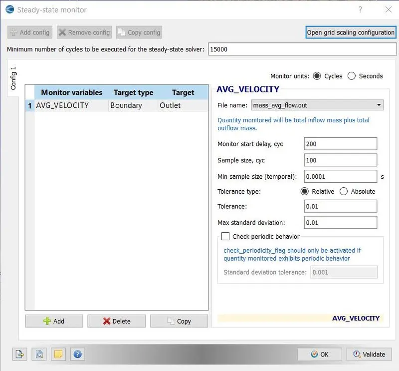
4. In steady state monitor average velocity with target type – boundary and target – outlet was selected.

Steady state monitor -

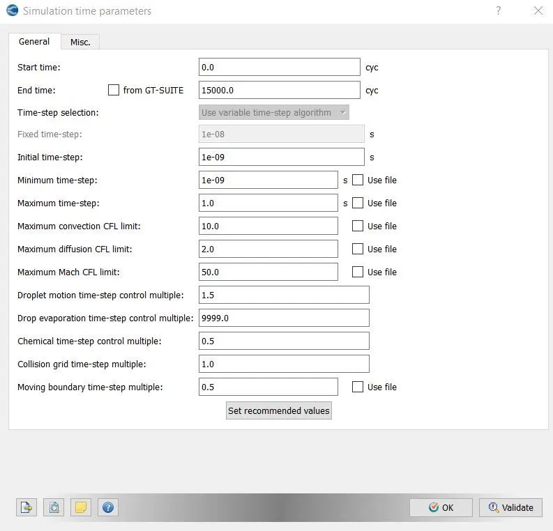
5. In simulation time parameter start time 0cycle, end time 15000cycle, initial time step - 1e-09s, minimum time step – 1e-09s, maximum time step 1s was chosen.

Time parameter -

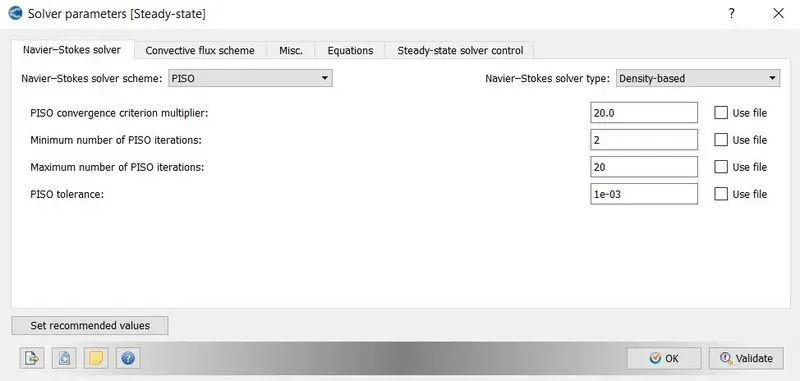
6. In solver parameters density-based solver was chosen which is a type of steady state solver, other parameters kept unchanged.

Solver Parameter -

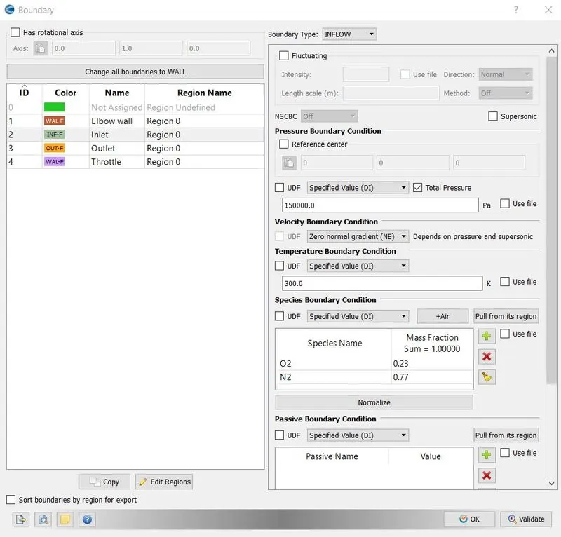
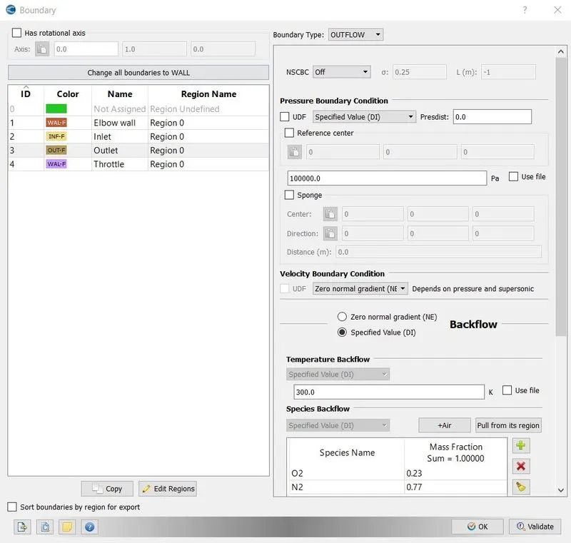
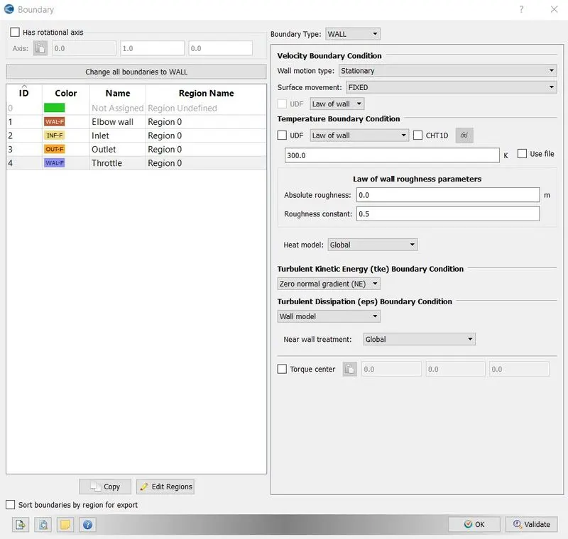
7. In boundary conditions Elbow wall, inlet, outlet and throttled was defined. Inlet was set with pressure value of 1.5e+05, similarly outlet was set with 1e+05. Throttle and elbow wall was fixed with law of wall. Air was fluid so it was also selected in inflow and outflow.

Boundary conditions -

Inlet -

Outlet -

Elbow wall -

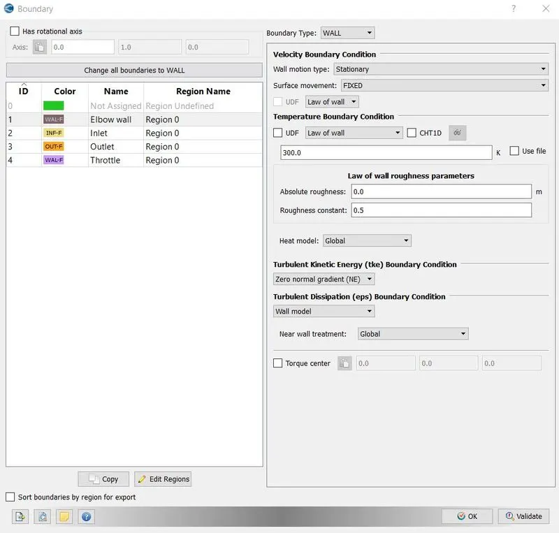
Trottle -

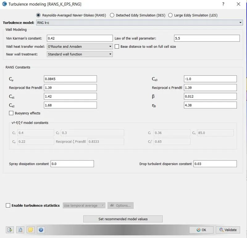
8. We went with default turbulence model which was Reynolds Averaged Navier Stokes k-epsilon model.

Turbulence model -

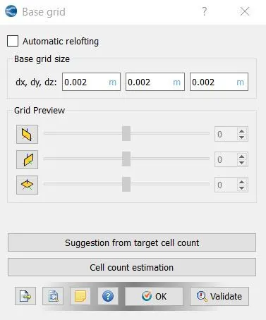
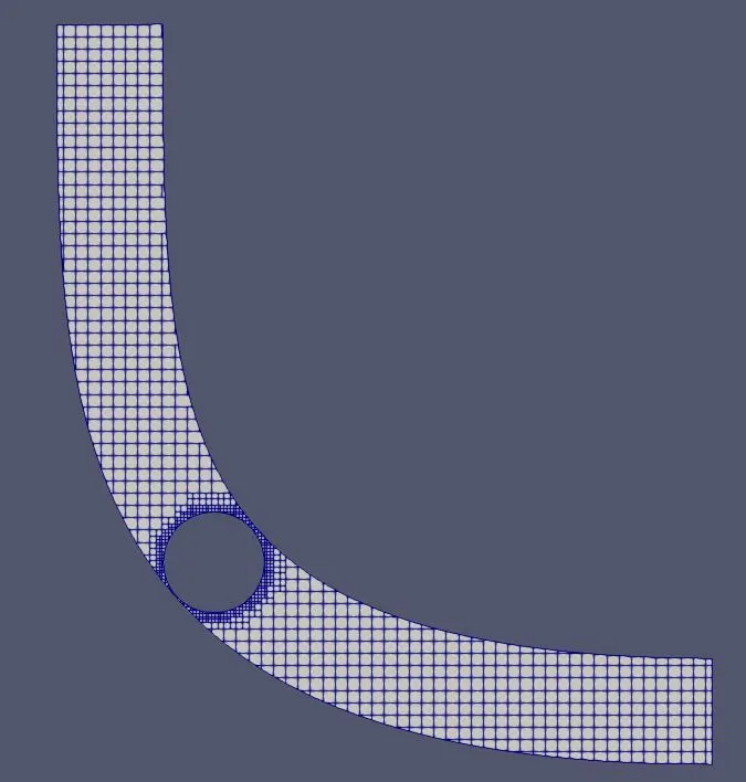
9. In grid control fixed embedding was enabled to get finer mesh near defined area. Grid size was set to 0.002m.

Grid size -

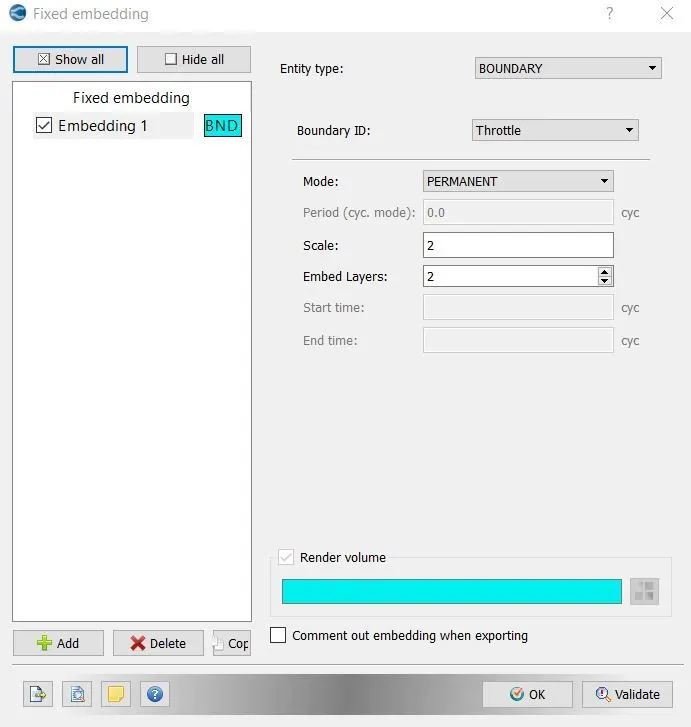
10. We wanted finer mesh around throttle, in fixed embedding boundary selected as throttle with mode permanent. Scale was selected as 2 means we got 0.001m mesh near throttle. Embedded layer was set at 2, which added 2 layers to the boundary.

Fixed embedding parameters-

11. Post variable selection allows us to select variables which we want to analyse in post processor. Converge has some variables as defaults, so went unchanged.

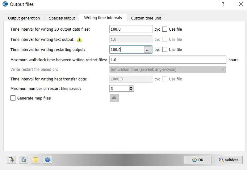
12. In output files 100 cycles were given as time interval to write 3D outputs and restarting output.

13. Input files exported in a folder and these solved using Cygwin terminal.

14. Files were converted into converge 3D postprocessing option and postprocessed in Paraview.

5. Results –

Mesh -

Velocity contour –

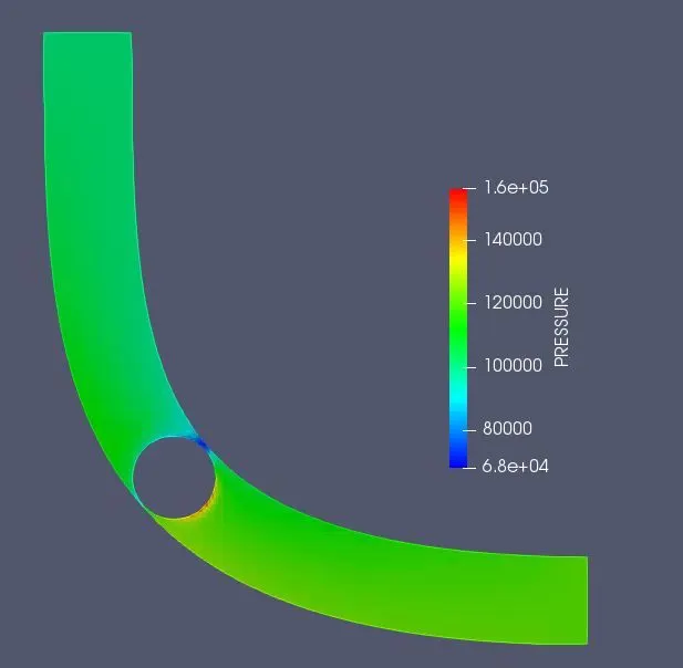
Pressure contour –

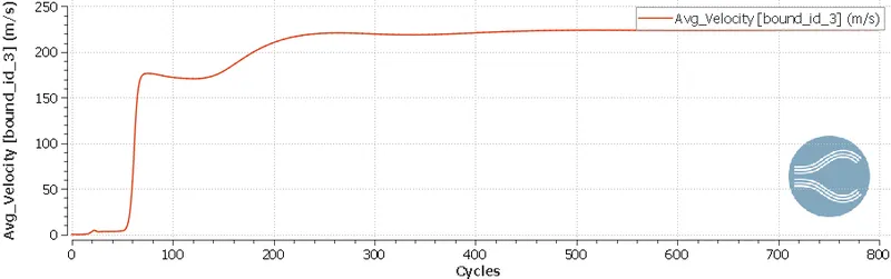
Velocity plot –

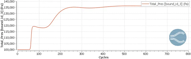
Pressure plot-

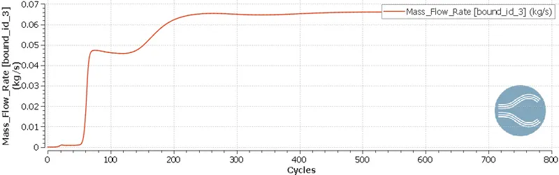
Mass flow rate –

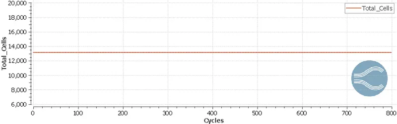
Cell count –

Animation -

https://drive.google.com/file/d/1bSchKUXaDQy1liXfTfJm6UiKVR0dpQxa/view?usp=sharing

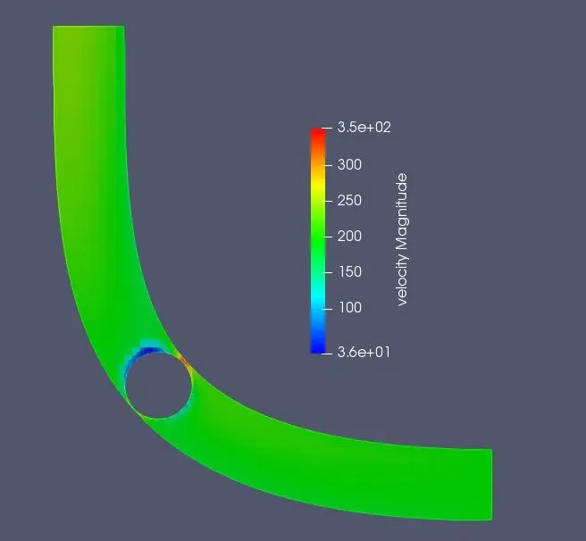
Pressure and velocity contour has created to visualize high pressure and maximum velocity areas, the contour is also help us to see area around, means how throttle is affecting fluid flow. Besides them, velocity, pressure, mass flow rate and cell count plot also created. Values of these parameters are fluctuating at beginning of simulation but after some cycles these are getting steady values. Pressure difference is the only cause of fluid flow here, we got values at outlet(maximum) – velocity -223.9m/s, pressure – 36287pa, mass flow rate -0.066kg/s.

6. Conclusion –

The steady state simulation of flow over throttle body has performed and inferred some results, although throttle was stationary. Results are validating theory, like we see velocity contour we can find the effect of throttle body, it is working as an obstacle and in narrower region velocity is maximum and fluid layers adjacent to throttle possess zero velocity, because here fluid particle is colliding with throttle and losing momentum. Similarly, pressure is low where velocity is high. We can conclude that throttle design, area around throttle affects the results most.