Genetic Algorithm

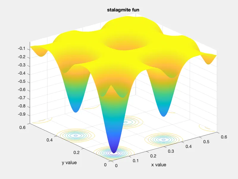
Creating a stalagmite function

%stalagmite function
function [f]=stalagmite(input_vector)

a=input_vector(1);
b=input_vector(2);

term1=(sin((3.5*pi*a)+0.8))^4;
term2=exp(-2*log(2)*((a-0.042)^2)/0.4);
term3=(sin((3.5*pi*b)+0.8))^4;
term4=exp(-2*log(2)*((b-0.042)^2)/0.4);

[f]=(term1*term2*term4*term3);
end

Since the inbuilt ga function in Matlab finds only optimizes for the minimum values, to maximize the function we can use the negative sign in the function.

%stalagmite function
function [f]=stalagmite(input_vector)

a=input_vector(1);
b=input_vector(2);

term1=(sin((3.5*pi*a)+0.8))^4;
term2=exp(-2*log(2)*((a-0.042)^2)/0.4);
term3=(sin((3.5*pi*b)+0.8))^4;
term4=exp(-2*log(2)*((b-0.042)^2)/0.4);

[f]=-(term1*term2*term4*term3);  % this is a maximization problem
end

Here is the code for solving the stalagmite function through genetic algorithm

%genetic algorithm
clear all
close all
clc


%defining search space
x=linspace(0,0.6,150);
y=linspace(0,0.6,150);

%generating a 2d mesh
[xx,yy]=meshgrid(x,y);

%no. of iterations
num_i=50;

for i=1:length(xx)
    for j=1:length(yy)
        input_vector(1)=xx(i,j);
        input_vector(2)=yy(i,j);
        f(i,j)=stalagmite(input_vector);
    end
end

surfc(xx,yy,f)
%surface creating
shading interp
xlabel('x value')
ylabel('y value')
title('stalagmite fun')

%study 1
tic
for i=1:num_i
    [xi,fval(i)]=ga(@stalagmite,2);
    xval(i)=xi(1);
    yval(i)=xi(2);
end
study1=toc
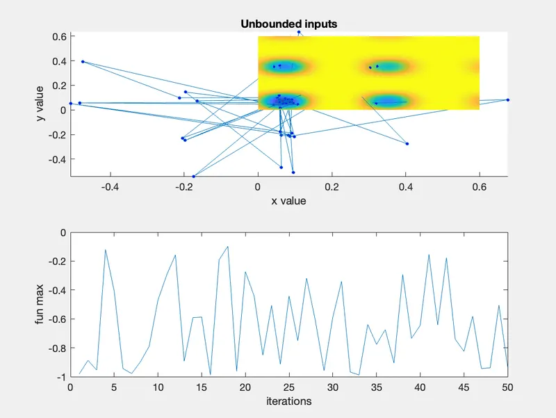
figure(2)

subplot(2,1,1)
hold on
surfc(x,y,f)
title('Unbounded inputs')
xlabel('x value')
ylabel('y value')
shading interp
hold on
%3D plotting 
plot3(xval,yval,fval,'Marker','o','MarkerSize',3,'MarkerFaceColor','b')

subplot(2,1,2)
plot(fval)
xlabel('iterations')
ylabel('fun max')

%study 2 with upper and lower bounds
tic;
for i=1:num_i
    [xi,fval(i)]=ga(@stalagmite,2,[],[],[],[],[0;0],[0.6;0.6]);
    xval(i)=xi(1);
    yval(i)=xi(2);
end
study2=toc
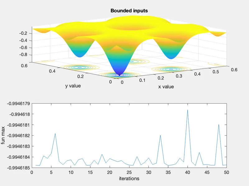
figure(3)
subplot(2,1,1)
surfc(x,y,f)
shading interp
title('Bounded inputs')
xlabel('x value')
ylabel('y value')
hold on
plot3(xval,yval,fval,'Marker','o','MarkerSize',3,'MarkerFaceColor','b')
subplot(2,1,2)
plot(fval)
xlabel('iterations')
ylabel('fun max')

%study 3 increasing population size
opt=optimoptions(@ga)
opt=optimoptions(@ga,'PopulationSize',1000)

tic
for i=1:num_i
    [xi,fval(i)]=ga(@stalagmite,2,[],[],[],[],[0;0],[0.6;0.6],[],[],opt);
    xval(i)=xi(1);
    yval(i)=xi(2);
end
study3=toc
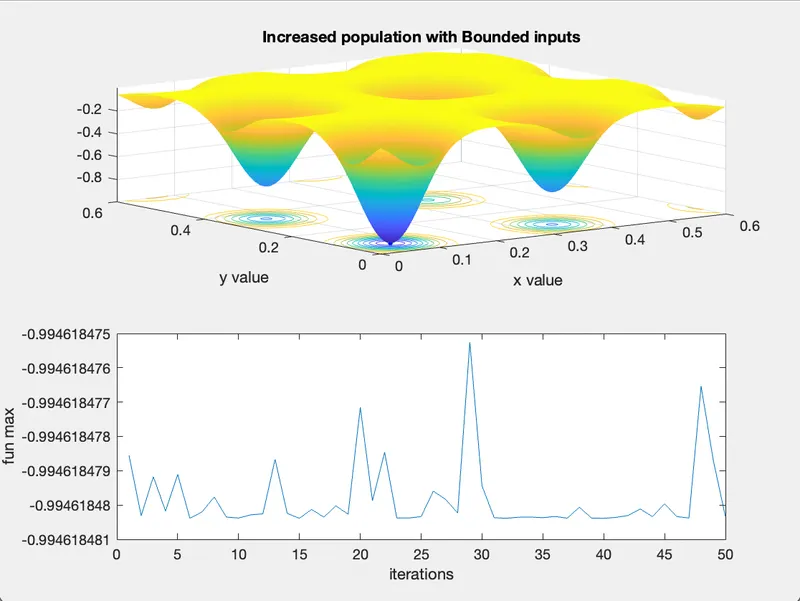
figure(4)
subplot(2,1,1)
surfc(x,y,f)
shading interp
title('Increased population with Bounded inputs')
xlabel('x value')
ylabel('y value')

hold on
plot3(xval,yval,fval,'Marker','o','MarkerSize',3,'MarkerFaceColor','b')
subplot(2,1,2)
plot(fval)
xlabel('iterations')
ylabel('fun max')

Here are the plots