Rankine cycle Simulator

Aim:

To simulate Rankine Cycle.

Objectives:

• To calculate the state points of the Rankine Cycle.
• To plot the corresponding T-s and h-s plots.

Theory:

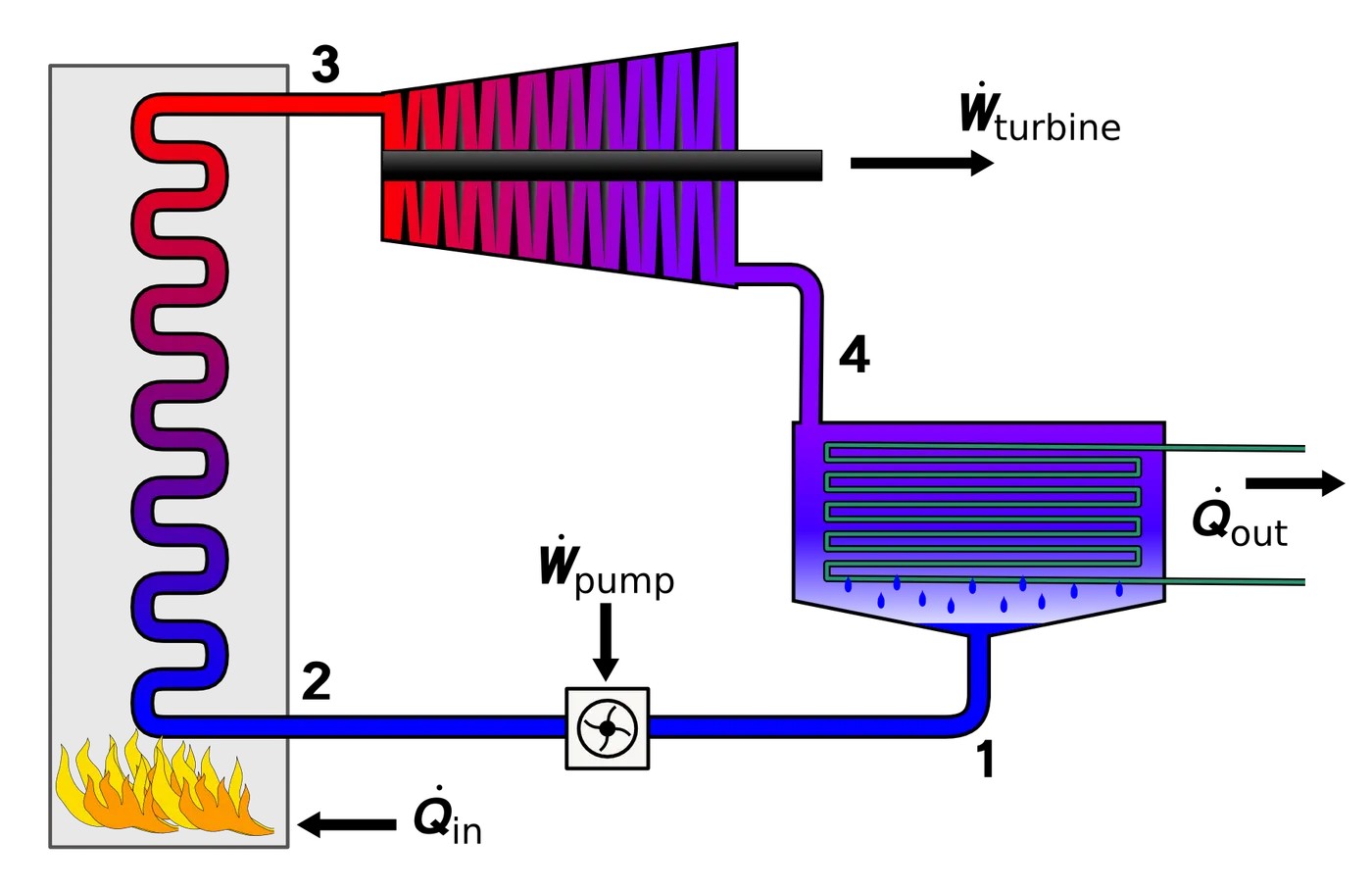
Rankine Cycle: The Rankine cycle is an idealized thermodynamic cycle describing the process by which certain heat engines, such as steam turbines or reciprocating steam engines, allow mechanical work to be extracted from a fluid as it moves between a heat source and heat sink.

Process:

1-2: Isentropic compression in the pump.

2-3: Constant pressure heat addition in the boiler.

3-4: Isentropic expansion in turbine.

4-1: Constant pressure heat rejection in the condenser.

Code:

clear all
close all
clc


%inputs
T1=400;
p1=30;
p2=0.05;


%stage 1 (turbine)
s1=XSteam('s_pT',p1,T1);
h1=XSteam('h_pT',p1,T1);

%stage 2 (condencer)
sf2=XSteam('sL_p',p2);
sg2=XSteam('sV_p',p2);
hf2=XSteam('hL_p',p2);
hg2=XSteam('hV_p',p2);

s2=s1;
T2=XSteam('Tsat_p',p2);

x2=((s2-sf2)/(sg2-sf2));
h2=hf2+(x2*(hg2-hf2));

%stage 3 (pump)
p3=p2;
T3=XSteam('Tsat_p',p2);
s3=XSteam('sL_p',p3);
h3=XSteam('hL_p',p3);

cp4=XSteam('cpL_p',p3);
cv4=XSteam('cvL_p',p3);
gamma=(cp4/cv4);
g=(gamma-1)/gamma;

%stage 4 (boiler)
p4=p1;
s4=s3;
h4=XSteam('h_ps',p4,s4);
T4=T3*((p4/p3)^g);

%work done by the turbine
wt=h1-h2;
%work done on the pump
wp=h4-h3;
%net work done
W=wt-wp;

%heat absorbed by the system
q1=h1-h4;
%heat rejected by the system
q2=h2-h3;

%efficiency
n=W/q1;
N=n*100;


SSC=3600/W;
tf=XSteam('Tsat_p',p1);
sf=XSteam('sL_p',p1);
hf=XSteam('hL_p',p1);
sg=XSteam('sV_p',p1);
hg=XSteam('hV_p',p1);

%plotting T-S diagram
figure(1)
hold on
temp=linspace(0,400,1000);
for i=1:length(temp)
    aa(i)=XSteam('sL_T',temp(i));
    bb(i)=XSteam('sV_T',temp(i));
end

plot(aa,temp,'Color','b')
plot(bb,temp,'Color','b')


temp=XSteam('Tsat_p',p1);
t=linspace(temp,T1,300);
for i=1:length(t)
    cc(i)=XSteam('s_pt',p1,t(i));
end

T5=XSteam('Tsat_p',p4);
s5=XSteam('sL_T',T5);

plot([s1 s2],[T1 T2],'Color','r')
plot([s2 s3],[T2 T3],'Color','r')
plot([s3 s4],[T3 T4],'Color','r')
plot([s4 s5],[T4 T5],'Color','r')
plot([sf sg],[tf tf],'Color','r')
plot(cc,t,'Color','r')

title('T-S Diagram')
xlabel('entropy')
ylabel('temperature')

text(s1,T1,'1');
text(s2,T2,'2');
text(s3,T3,'3');
text(s4,T4,'4');
text(s5,T5,'4s');
text(sg,tf,'1s');

%plotting H-S diagram
figure(2)
hold on

temp2=linspace(0,400,1000);
for i=1:length(temp2)
    dd(i)=XSteam('hL_T',temp2(i));
    ee(i)=XSteam('hV_T',temp2(i));
end

plot(aa,dd,'Color','b')
plot(bb,ee,'Color','b')

plot([s1 s2],[h1 h2],'Color','r')
plot([s2 s3],[h2 h3],'Color','r')
plot([s3 s4],[h3 h4],'Color','r')
plot([s4 s1],[h4 h1],'Color','r')

title('H-S Diagram')
xlabel('entropy')
ylabel('enthalpy')

%printing the results
fprintf('At stage1: n')
fprintf('P1=%f bar n T1=%f degree celcius n H1=%f kJ/kg n S1=%f kJ/kg-k n',p1,T1,h1,s1)

fprintf('At stage2: n')
fprintf('P2=%f bar n T2=%f degree celcius n H2=%f kJ/kg n S2=%f kJ/kg-k n',p2,T2,h2,s2)

fprintf('At stage3: n')
fprintf('P3=%f bar n T3=%f degree celcius n H3=%f kJ/kg n S3=%f kJ/kg-k n',p3,T3,h3,s3)

fprintf('At stage4: n')
fprintf('P4=%f bar n T4=%f degree celcius n H4=%f kJ/kg n S4=%f kJ/kg-k n',p4,T4,h4,s4)

fprintf('Work done by the turbine=%f kJ/kg n',wt)
fprintf('Work done on the pump=%f kJ/kg n',wp)
fprintf('Net work done by the system=%f kJ/kg n',W)
fprintf('Thermal efficiency of the system=%f %% n',N)
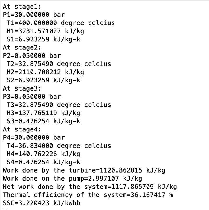
fprintf('SSC=%f kJ/kWhb n',SSC)

Results:

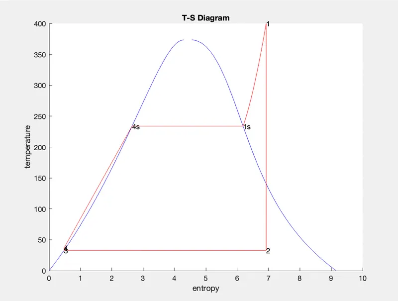
T-S Diagram

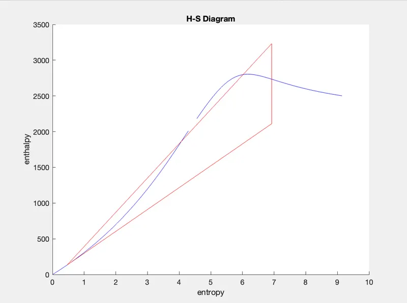
H-S Diagram

Output Screen: