Week 4.1 - Genetic Algorithm

Aim: to write a program for stalagmite function and find its global maxima using genetic algorithm.

Governing equations:

`f(y1)=[sin(5.1*pi*y+0.5)]^6`

`f(y2)=exp((-4*ln(2)*((y-0.0667)^2)/0.64))`

`f(x1)=[sin(5.1*pi*x+0.5)]^6`

`f(x2)=exp(-4*ln(2)*(((x-0.0667)^2))/0.64)`

`f(x,y)=f(y1)*f(y2)*f(x1)*f(x2)`

The function consists of 4 values two of which are derived from ‘x’ and the other two from ‘y’.

Objectives: optimise the stalagmite function , find its global maxima , explain GA and its syntax.

Body:

Theory:

Stalagmite function :

Stalagmite function is a function with a lot of local maximas and local minima that resemble the stalagmites formed naturally in a cave.

When we inverse the function using the minus sign at the result , we form the stalactite function which resembles the stalactites that are formed in the cave just above stalagmites.

Genetic algorithm:

Genetic algorithm is a method for solving optimisation problems that is based on natural selection which is based of Charles Darwins theory of biological evolution. If parents have better fitness, their offspring will be better than parents and have a better chance at surviving. This process keeps on iterating and at the end, a generation with the fittest individuals will be found.

Five phases are considered in a genetic algorithm.

• Initial population
• Fitness function
• Selection
• Crossover
• Mutation

Syntax of GA:

x = ga(function,nvars) finds a local unconstrained minimum, x, to the objective function, function. nvars is the dimension (number of design variables) of function

x = ga(function,nvars,A,b) finds a local minimum x to function, subject to the linear inequalities A*x ≤ b. ga evaluates the matrix product A*x as if x is transposed (A*x').

.

x = ga(function,nvars,A,b,Aeq,beq) finds a local minimum x to function, subject to the linear equalities Aeq*x = beq and A*x ≤ b. (Set A=[ ] and b=[ ] if no linear inequalities exist.) ga evaluates the matrix product Aeq*x as if x is transposed (Aeq*x').

.

x = ga(function,nvars,A,b,Aeq,beq,lb,ub) defines a set of lower and upper bounds on the design variables, x, so that a solution is found in the range lb ≤ x ≤ ub. (Set Aeq=[ ] and beq=[ ] if no linear equalities exist.)

.

x = ga(function,nvars,A,b,Aeq,beq,lb,ub,nonlcon) subjects the minimization to the constraints defined in nonlcon. The function nonlcon accepts x and returns vectors C and Ceq, representing the nonlinear inequalities and equalities respectively. ga minimizes the function such that C(x) ≤ 0 and Ceq(x) = 0. (Set lb=[ ] and ub=[ ] if no bounds exist.)

.

x = ga(function,nvars,A,b,Aeq,beq,lb,ub,nonlcon,options) minimizes with the default optimization parameters replaced by values in options. (Set nonlcon=[ ] if no nonlinear constraints exist.) Create options using optimoptions.

.

x = ga(function,nvars,A,b,Aeq,beq,lb,ub,nonlcon,intcon) or x = ga(function,nvars,A,b,Aeq,beq,lb,ub,nonlcon,intcon,options) requires that the variables listed in intcon take integer values.

This syntax has been copied from the help centre of matlab

From all these syntaxes

We have used the following one to complete our program:

x = ga(fun,nvars,A,b,Aeq,beq,lb,ub,nonlcon,options)

code:

close all 
clear vars 
clc 

%defining x and y variables
x=linspace(0,0.6,150);
y=linspace(0,0.6,150);
num_cases=50;
[xx,yy]=meshgrid(x,y);

for i=1:length(xx)
    for j=1:length(xx)

        
%getting values for input vector
       inputvector(1)=xx(i,j);
       inputvector(2)=yy(i,j);
       f(i,j)=stalagmite(inputvector);
    end 

end


%1st study

%getting the value for f using the stalagmite function 
        
       
        %getting different values for f(val) in 50 cases
for k=1:num_cases 
    [input,fval(k)]= ga(@stalagmite,2);
    xopt(k)=input(1);
    yopt(k)=input(2);

end 

%plotting different graphs for stalagmite function and dofferent values of
%fval

figure(1)
subplot(2,1,1)
hold on
surfc(x,y,f)
shading interp
plot3(xopt,yopt,fval,'marker','o','markersize',5,'markerfacecolor','r')
title('unbounded inputs')
subplot(2,1,2)
plot(fval)
xlabel('iterations')
ylabel('function value')

   


%2nd study

for k=1:num_cases 
    [input,fval(k)]= ga(@stalagmite,2,[],[],[],[],[0;0],[1;1],[],[],options); %giving boundary conditions for the stalagmite function 
    xopt(k)=input(1);
    yopt(k)=input(2);

end 


%plotting different graphs for stalagmite function and dofferent values of
%fval

figure(2)
subplot(2,1,1)
hold on
surfc(x,y,f)
shading interp
plot3(xopt,yopt,fval,'marker','o','markersize',5,'markerfacecolor','r')
title('unbounded inputs')
subplot(2,1,2)
plot(fval)
xlabel('iterations')
ylabel('function value')   



%3rd study 
%defining another parameter for stalagmite and putting opulation size as 300 
        options=optimoptions('ga');
        options=optimoptions(options,'PopulationSize',300);
   

for k=1:num_cases 
    [input,fval(k)]= ga(@stalagmite,2,[],[],[],[],[0;0],[1;1],[],[]); %giving boundary conditions for the stalagmite function
    xopt(k)=input(1);
    yopt(k)=input(2);

end 



%plotting different graphs for stalagmite function and dofferent values of
%fval

figure(3)
subplot(2,1,1)
hold on
surfc(x,y,f)
shading interp
plot3(xopt,yopt,fval,'marker','o','markersize',5,'markerfacecolor','r')
title('unbounded inputs')
subplot(2,1,2)
plot(fval)
xlabel('iterations')
ylabel('function value')

stalagmite function code:

function[V]= stalagmite(inputvector)
x=inputvector(1);
y=inputvector(2);
y1=(sin(5.1*pi*y+0.5)).^6;
y2=exp((-4*log(2)*(((y-0.0667)^2))/0.64));
x1=(sin(5.1*pi*x+0.5)).^6;
x2=exp((-4*log(2)*(((x-0.0667)^2))/0.64));

V=-(x1*y1*x2*y2);


end

Code explanation:

• First we define the vales for x and y using linspace command(0 to 0.6 with 150 data points)
• Defining the number of cases to be 50.
• Using for command to iterate ‘i ’ from 1 to the length of xx i.e 150.
• Using for command to iterate ‘j’ from 1 to the length of xx i.e 150.
• We use a nested if loop so that we get all the values for x(i,j) and j(i ,j).
• Storing the i ,jth value of of xx in inputvector(1) and i ,jth value of yy in inputvector(2).
• And using these 2 values of inputputvector to get all the values of ‘f’.

1st study

• Using another for loop ‘k’ from 1 to number of cases i .e 50.
• Getting the values for the maxima of stalagmite using an inbuilt solver called ga (genetic algorithm).
• The points where the maxima is formed is stored in input variable.
• And the maximum point of stalagmite will be stored in f(val).
• Storing the first value of input vector for every kth iteration in x-opt.
• Storing the second value of input vector for every kth iteration in y-opt.
• Plotting figure(1)
• Making a subplot with dimensions(2,1,1)
• Using hold on command to get several plots together
• Using surface commas to get the stalagmite function plot surface
• Shading interp command to omit all the lines denoting the data points in order to get a cleaner surface.
• Plot3 command plots all the data points in 3d and hence uses 3 inputs. Which is xopt ,yopt and and fval in this case.
• The title command gives the title of unbounded inputs to the first plot.
• Creating another subplot with dimensions (2,1,2)
• Plotting the values of fval in this subplot.
• Labelling x axis as iterations
• Labelling y axis as function value
• We do another study because we get different values for fval with very high tolerance and thesis not ideal.

2nd study

• Using for loop ‘k’ from 1 to number of cases i .e 50.
• Th only change in this study is that we are giving boundary conditions for the GA solver. That is from 0,0 to 1,1.
• This means that the value of fval can only exist between 0,0 and 1,1.
• This will narrow down our result and will give us consistent values.
• The rest of the code is totally same as time study 1.
• We do another study as the results are still a lil inconsistent.

3rd study

• In this study we are using options command that is used to give conditions for GA.
• We are defining the population size to be 300.
• This will give more initial population for ga to solve. That will Give us even more consistent results.
• The rest of the code is same as study 2.

Stalagmite function code

• Defining a function ‘stalagmite’ with pointer ‘A’ taking input from variable ‘inputvector’.
• This function will be called in the program genetic_algorithm for every iteration of nested loop i and j.
• Storing the first value of inputvector in x
• Storing the second value of inputvector in y
• Getting the values of y1 , x1 , y2, x2 using the equation mentioned above.
• The final value of the function is -(x1*y1*x2*y2)
• We are using the negative value of the function in order to invert the graph of the stalagmite function.
• Since we have inverted the whole function , now when we will use GA it will give us the maximum value since the function is inverted.

results:

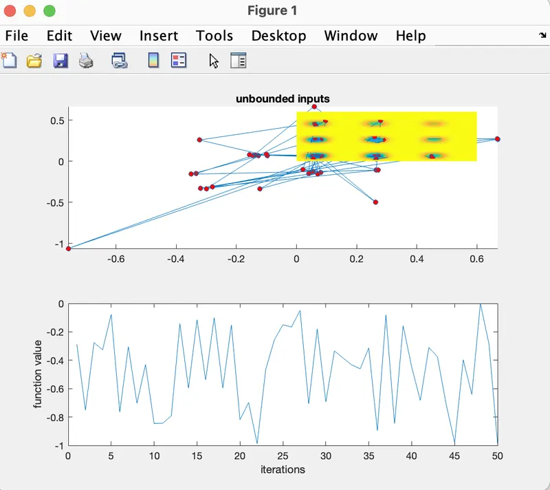
as we can see there are a lot of different values for the function. we cannot decern the maximum value for the function like this.

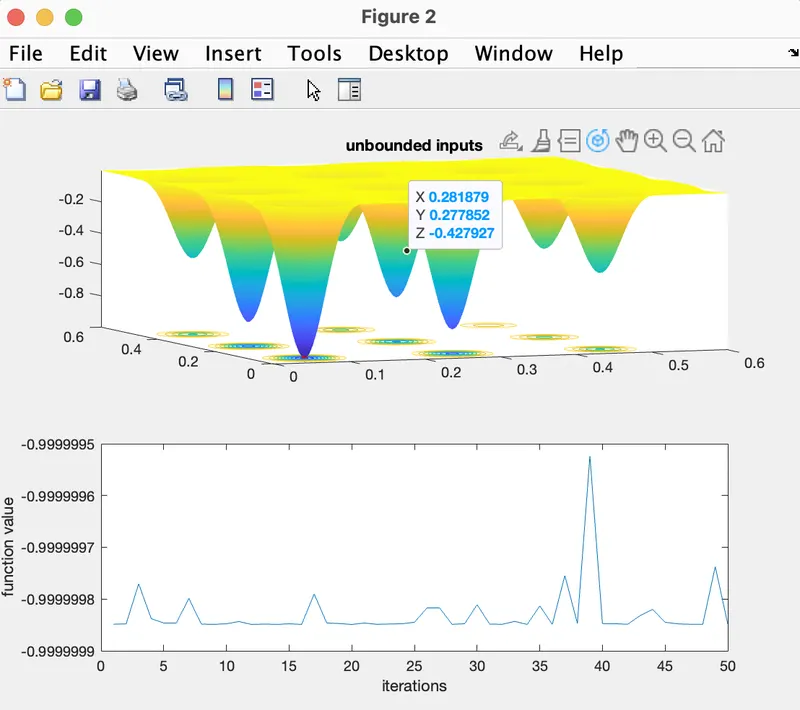
even is this study the value of function varies. the marker gives only one data point though.

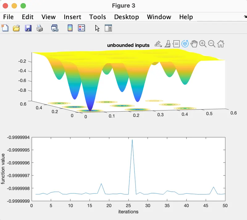
this study gives consistent results and onlyone data point on the stalagmite function as we can see in the graph.

References: https://towardsdatascience.com/introduction-to-genetic-algorithms-including-.-code-e396e98d8bf3

https://www.geeksforgeeks.org/genetic-algorithms/

Errors: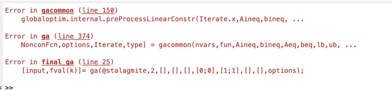

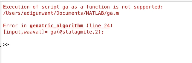
the error was due to the wrimg syntax of ga solver.

I was missimg one [ ], due tp which matlabw as not able to put boundary conditionss

the second error was due to the program being saved as ga due to which matlab was not able to use the solver ga.

conclusion.

the program was written and the results were carried out. study 3 gives the best results and the most consistent ones too.

the limitation is that ga doesnt give the perfect result everytime byt the tolerance is verry less due to which the result is verry close to the real maxima.