Week 4.1 - Genetic Algorithm
Aim:
To write a MATLAB code to optimize the stalagmite function and find the global maxima of the function.
Algorithm:
- A coordinate system is first initialized to fix the working space of the function using the genetic algorithm.
- The number of iterations is decided and initialized within the input initialization part of the program
- The stalagmite function is defined in a separate file as per its mathematical definition.
- The stalagmite function is called in the main function and the mesh grid generated in the main program is initialized for the stalagmite function using the loop function of the Matlab.
- Next is the initialization of the three cases as per the use of the genetic algorithm.
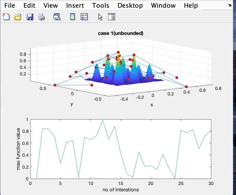
- The three cases will be according to the syntax of the genetic algorithm. These cases are the unbounded case, bounded case, and lastly optimized function bounded case.
- Each case will have plot commands generating the various contours for the visual representation of the global maxima that has to be found out using this program
MAIN CODE:
% start of the program
close all
clear all
clc
x=linspace(0,0.6,150);
y=linspace(0,0.6,150);
limit=30;
%creating 2D array using meshgrid function
[xx yy]=meshgrid(x,y);
%nested loop for array value input
for i=1: length(xx)
for j=1:length(yy);
input_vector(1)=xx(i,j);
input_vector(2)=yy(i,j);
f(i,j)= stalagmite(input_vector);
end
end
tic
for i=1: limit
[input,fval(i)]=ga(@stalagmite,2);
x_out(i)=input(1);
y_out(i)=input(2);
end
case_time_1=toc;
figure(1)
subplot(2,1,1)
surfc(xx,yy,-f)
xlabel('x')
ylabel('y')
title('case 1(unbounded)','Color','k')
shading interp
hold on
plot3(x_out,y_out,-fval,'marker','o','MarkerSize',6,'MarkerFaceColor','r');
subplot(2,1,2)
plot(-fval);
xlabel('no of Interations')
ylabel('max function value')
%case :2 Inserting bounding box
tic
for i=1: limit
[input,fval(i)]=ga(@stalagmite,2,[],[],[],[],[0;0],[0.6;0.6]);
x_out(i)=input(1);
y_out(i)=input(2);
end
case_time_2=toc;
figure(2);
subplot(2,1,1)
hold on;
surfc(xx,yy,-f)
xlabel('x')
ylabel('y')
title('case 2','Color','k')
shading interp
plot3(x_out,y_out,-fval,'marker','o','MarkerSize',6,'MarkerFaceColor','r');
subplot(2,1,2)
plot(-fval)
xlabel('no of Interations')
ylabel('max function value')
%case:3
options=optimoptions(@ga)
options=optimoptions(options,'populationsize',170);
tic
for i=1: limit
[input,fval(i)]=ga(@stalagmite,2,[],[],[],[],[0;0],[0.6;0.6],[],[],options);
x_out(i)=input(1);
y_out(i)=input(2);
end
case_time_3=toc;
figure(3)
subplot(2,1,1)
hold on
surfc(xx,yy,-f)
shading interp
xlabel('x');
ylabel('y');
title('case 3','Color','k')
plot3(x_out,y_out,-fval,'marker','o','MarkerSize',6,'MarkerFaceColor','r');
subplot(2,1,2)
plot(-fval);
xlabel('no of Interations')
ylabel('max function value')
%case:4
options=optimoptions(@ga)
options=optimoptions(options,'populationsize',300);
tic
for i=1: limit
[input,fval(i)]=ga(@stalagmite,2,[],[],[],[],[0;0],[0.1;0.1],[],[],options);
x_out(i)=input(1);
y_out(i)=input(2);
end
case_time_4=toc;
figure(4)
subplot(2,1,1)
hold on
surfc(xx,yy,-f)
shading interp
xlabel('x');
ylabel('y');
title('case 4','Color','k')
plot3(x_out,y_out,-fval,'marker','o','MarkerSize',6,'MarkerFaceColor','r');
subplot(2,1,2)
plot(-fval);
xlabel('no of Interations')
ylabel('max function value')
%Displaying the values of x & y for maximum value of function
display(input)
%end of program
STALAGMITE FUNCTION :
%stalagmite function
function [f]= stalagmite(input_vector)
f1x= (sin((5.1*pi).*input_vector(1)+0.5)).^6;
f1y= (sin((5.1*pi).*input_vector(2)+0.5)).^6;
f2x= exp((((input_vector(1)-0.0667).^2)/0.64).*(-4*log(2)));
f2y= exp((((input_vector(2)-0.0667).^2)/0.64).*(-4*log(2)));
f1=f1x*f1y*f2x*f2y;
f=-f1;
end
Working of code:
- Create the coordinate system so that a mesh grid can be achieved using a linspace command in Matlab.
- Next is to fix and specify the number of total iterations that the program is required to complete so that global maxima can be calculated.
- Now the main function that will be utilized in the program is called by using the loop function on the generated mesh grid.
- Before calling the function, we have to create the function definition in the different files located in the same folder as that of the main program as per the mathematical equations mentioned in the challenge.
- Now the three cases according to the definition of the genetic algorithm function are executed using the loop feature of Matlab.
- The first case of the study of the genetic algorithm provides the statistical behavior of the function apart from the mesh that is defined as seen by the plot generated.
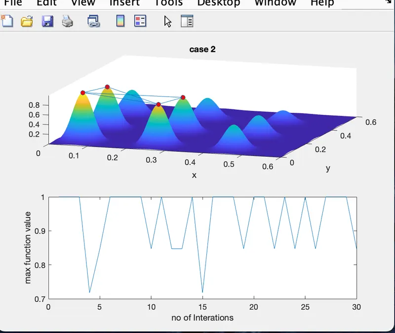
- The second study will be done so that the genetic algorithm can be utilized in between the mesh grid provided, for that the syntax of genetic algorithm that has lower and upper bounds will be utilized in the program.
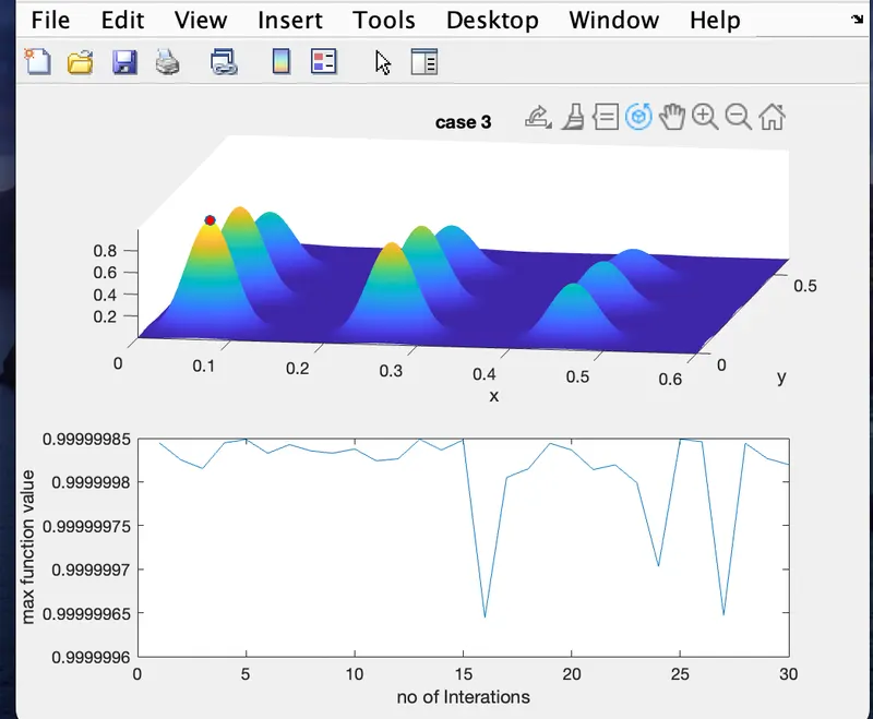
- Since the program is still unable to give a fixed input of the value of the global maxima of the function the optimization of the function using the genetic algorithm function is used.
- Each case study has an inbuilt plot generation command to monitor the number of iterations as well as fluctuations within the main program.
- Each case study also has a timer command in them to calculate the time elapsed during the running of each individual case within the program.
Learning:
- Genetic algorithm
The following outline summarizes how the genetic algorithm works:
- The algorithm begins by creating a random initial population.
- The algorithm then creates a sequence of new populations. At each step, the algorithm uses the individuals in the current generation to create the next population. To create a new population, the algorithm performs the following steps:
- Scores each member of the current population by computing its fitness value.
- Scales the raw fitness scores to convert them into a more usable range of values.
- Selects members, called parents, based on their fitness.
- Some of the individuals in the current population that have lower fitness are chosen as elite. These elite individuals are passed to the next population.
RESULT:
CASE:1(UNBOUNDED)
CASE :2(BOUNDED)
CASE:3 (BOUNDED WITH INCREASED POPULATION SIZE )
CASE:4(Bounded with more population size)
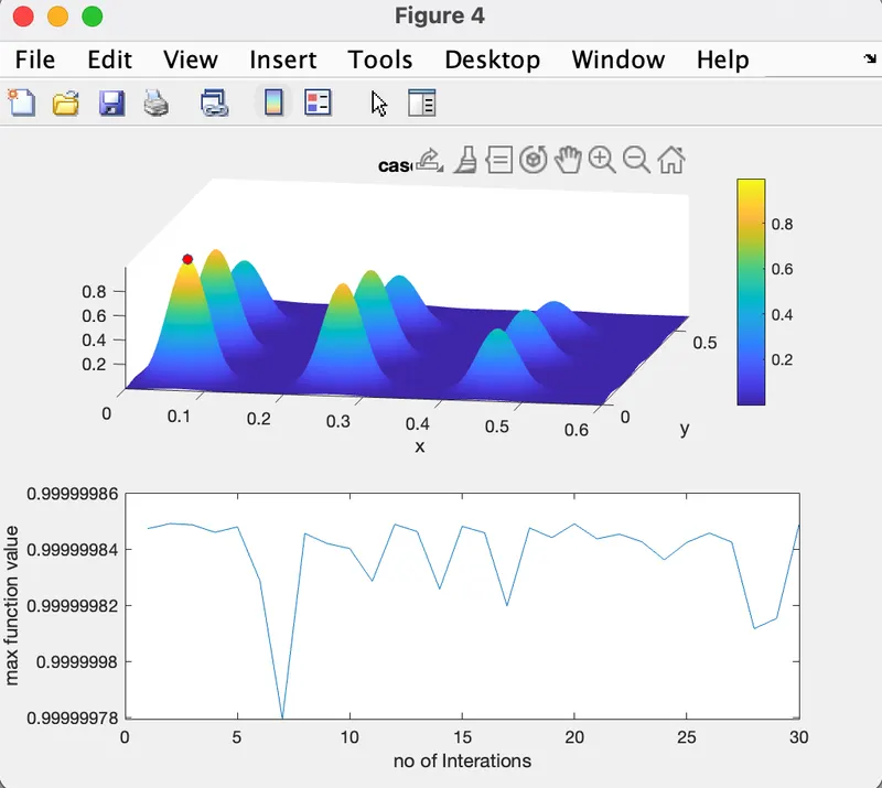
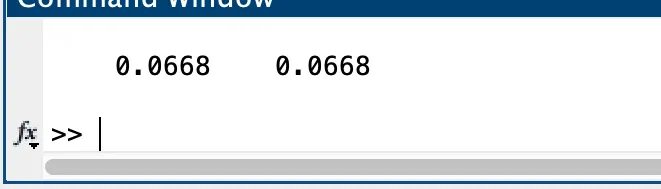
Value of x & y for maximum value of function