Challenge

Week 3 - Solving second order ODEs

HHarish N16 May 2022

AIM:

To solve the second-order ode function using Matlab which depicts the motion of the pendulum and to create an animation of the same.

OBJECTIVE:

To write a program that solves the following ODE. This ODE represents the equation of motion of a simple pendulum with damping

In the above equation,

g = gravity in m/s2,

L = length of the pendulum in m.

m = mass of the ball in kg,

b=damping coefficient.

FIXED PARAMETERS

Length (L) =1 metre,

Mass (m) =1 kg.

Damping colefficient (b) =0.05.

Acceleration due to gravity (g) =9.81 m/s2.

For Time period = 0-20 sec

Angular displacement=0, Angular velocity=3 rad/sec at time t=0.

FUNCTION CODE:

function [dtheta_dt] = ode_func(t,theta,b,g,l,m);

theta1 = theta(1);

theta2 = theta(2);

dtheta1_dt = theta2;

dtheta2_dt = -(b/m)*theta2 - (g/l)*sin(theta1);

dtheta_dt = [dtheta1_dt;dtheta2_dt];

end

MAIN PROGRAM:

close all

clear all

clc

% input

b = 0.05;

g =9.81;

l =1;

m =0.1;

% initial condition

theta_0 = [0;5];

%time points

t_span = linspace(0,10,500);

% solve ode

[t,results] = ode45(@(t,theta) ode_func(t,theta, b,g,l,m),t_span, theta_0);

plot(t,results(:,1))

hold on

plot(t,results(:,2))

xlabel('plote')

ylabel('time')

% animation

ct = 1

for i = 1: length(results(:,1))

x0 = 0;

y0 = 0;

x1 = 1*sin(results(i,1)+pi);

y1 = 1*cos(results(i,1)+pi);

figure(2)

plot([x0,x1],[y0,y1],'-o','MarkerSize',10,'MarkerFaceColor','r','MarkerEdgeColor','r','linewidth',4)

axis([-2 2 -2 2])

hold on

plot([-1 1],[0 0],'LineWidth',5,'Color','[0 0.3 0]')

M(ct) = getframe(gcf)

hold off

ct = ct + 1

end

% videofile

movie(M)

v_f = VideoWriter('pendulum_chelleng.avi','Uncompressed AVI')

open(v_f)

writeVideo(v_f,M)

close(v_f)

Detail explanation each step of the program:

1. In the first step Input and initial

condition of a simple pendulum is fed.

2. Then the program is written to solve the ODE in which Matlab inbuilt function (ode45) is used with constant theta, t, and another function is used, which is defined separately in the function program.

3. In the next step result of solved ODE is plotted w.r.t time using the plot command.

4. Now iteration of co-ordinate is fed using for loop to create animation.

5. Then plot command is used to plot the pendulum string and bob.

6. In the next step, the move command is used to create an animated video of the oscillating pendulum.

ERROR

have a small spelling mistake in the code and file saving code.

OUTPUT:

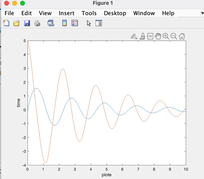
• A plot is drawn between the angular acceleration and displacement of the motion of the simple pendulum.

• The blue curve is the displacement where it starts from zero. And the angular velocity is starting at 3 (rad/sec).

• At the end of the t_span both the displacement and angular velocity becomes zero and the motion of a simple pendulum becomes zero which becomes the rest

PLOT:

ANIMATION:

https://youtu.be/VkdQGaATTIU

Week 3 - Solving second order ODEs

Ship work like this
in your own course.

Talk to a career counsellor

Ship work like thisin your own course.

Talk to a career counsellor

Ship work like this
in your own course.