Week 4.1 - Genetic Algorithm

Course: MATLAB for Mechanical Engineers

Challenge: Genetic Algorithm

Submitted By: Amanpreet Singh

1 Aim:

The aim of the week 4 challenge is to write a code in MATLAB to optimize the stalagmite function and find the global maxima of the function.

2 Objectives:

The objectives of the week 4 challenges are as follows:

• To gain an overall knowledge of the Genetic Algorithm for optimization and Stalagmite Function.
• Plot the graphs based on three studies performed for finding global maxima of the given function using MATLAB.

3 Theory:

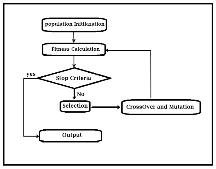
A genetic algorithm (GA) is a search-based optimization technique based on the principles of Genetics and Natural Selection. It is frequently used to find optimal or near-optimal solutions to difficult problems which otherwise would take a lifetime to solve. It is frequently used to solve optimization problems, in research, and in machine learning.

A genetic algorithm is a search heuristic that is inspired by Charles Darwin’s theory of natural evolution. This algorithm reflects the process of natural selection where the fittest individuals are selected for reproduction in order to produce offspring for the next generation.

The notion of Natural Selection

The process of natural selection starts with the selection of the fittest individuals from a population. They produce offspring which inherit the characteristics of the parents and will be added to the next generation. If parents have better fitness, their offspring will be better than their parents and have a better chance of surviving. This process keeps on iterating and in the end, a generation with the fittest individuals will be found.

This notion can be applied to a search problem. We consider a set of solutions for a problem and select the set of best ones out of them.

Five phases are considered in a genetic algorithm.

• Initial population
• Fitness function
• Selection
• Crossover
• Mutation

Stalagmite Function:

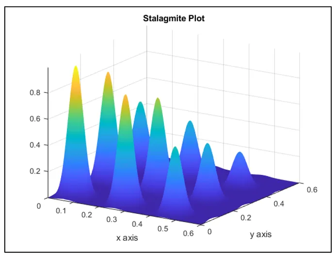
Stalagmite function is a mathematical model which helps to generate local minima and local maxima. It is a three-dimensional function designed in a way that results in multiple Local maxima or minima and only one Global maximum or global minima. The name stalagmite itself describes a type of rock formation that rises from the floor of the cave due to the accumulation of the material deposited on the floor from the ceiling drippings.

The Stalagmite function used in the MATLAB Code is as follows:

f(x,y) = f₁x f₂x f₁y f₂y

f₁x = (sin(5.1 π x +0.5))^0.6

f₁y = (sin(5.1 π y +0.5))^0.6

f₁y = exp (-4ln2* (x-0.0067)² / 0.64)

f₂y = exp (-4ln2* (y-0.0067)² / 0.64)

Syntax to be followed to define Genetic Algorithm (ga) in MATLAB:

The “ga” syntax in MATLAB is primarily used to find the minimum of the given function. There are multiple ways to define a “ga” syntax in MATLAB to solve an optimization problem. The syntax used for the completion of the challenge is as follows.

x = ga (fun, nvars); finds a local unconstrained minimum

where,

x is the optimal solution/variables

fun = objective function

nvars = no of variables

x = ga (fun, nvars, A, B, Aeq, Beq, lb, ub)

where,

A, B = Linear inequality constraints

Aeq, Beq = Linear equality constraints

If there are no linear equalities and inequalities, then A, B, Aeq, Beq are set to [].

x = ga (fun, nvars, A, B, Aeq, Beq, lb, ub, nonlcon, Intcon, options )

where,

nonlcon = Nonlinear constraints

Intcon = Integer Values

Options= Optimisation options

If there are no nonlinear constraints and Integer values, then nonlcon & Intcon are set to [].

Optimization Studies:

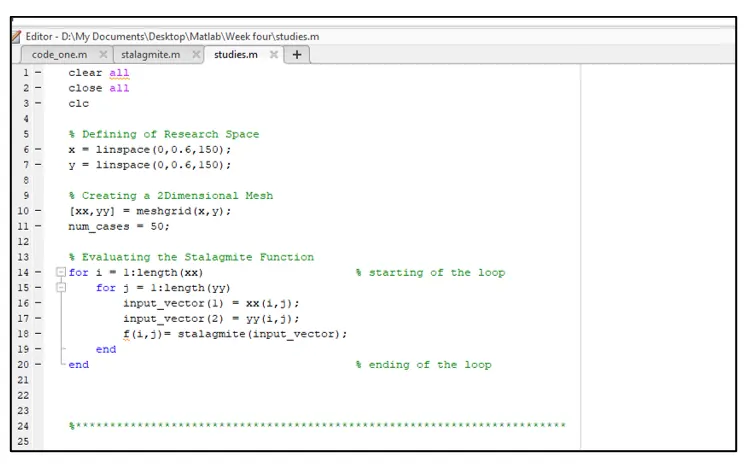
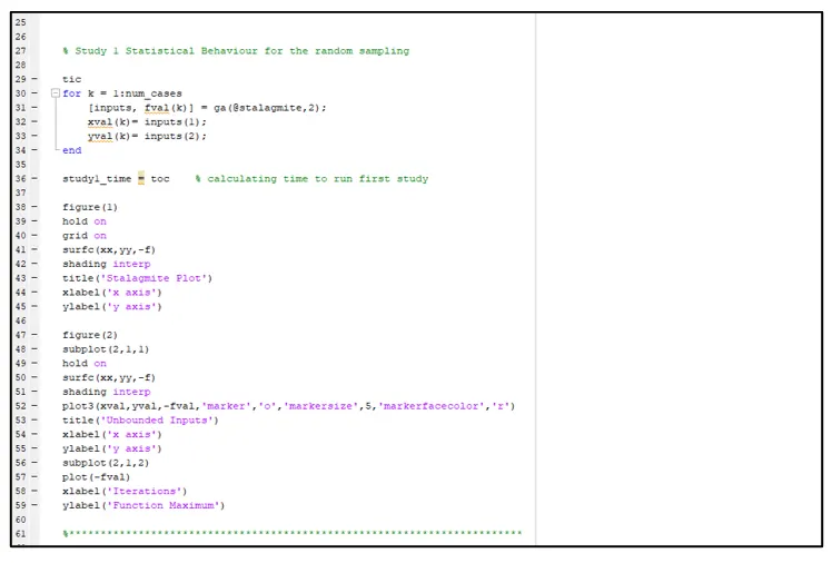
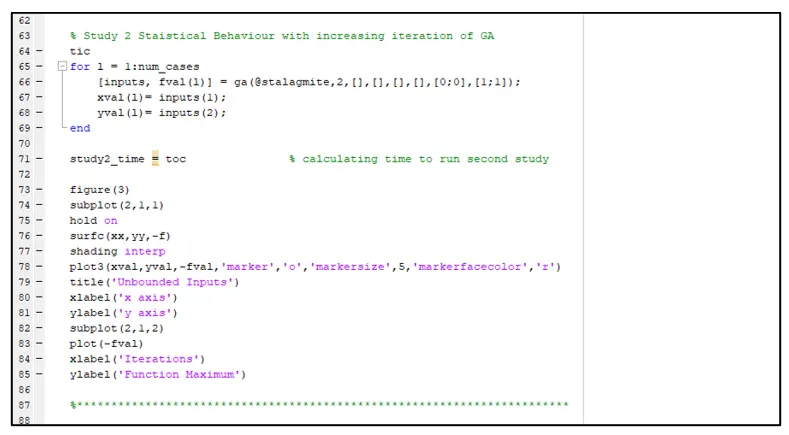
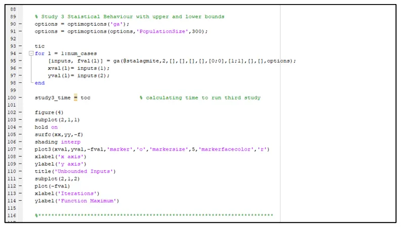
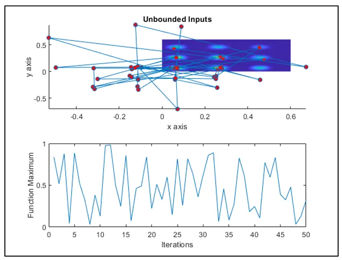
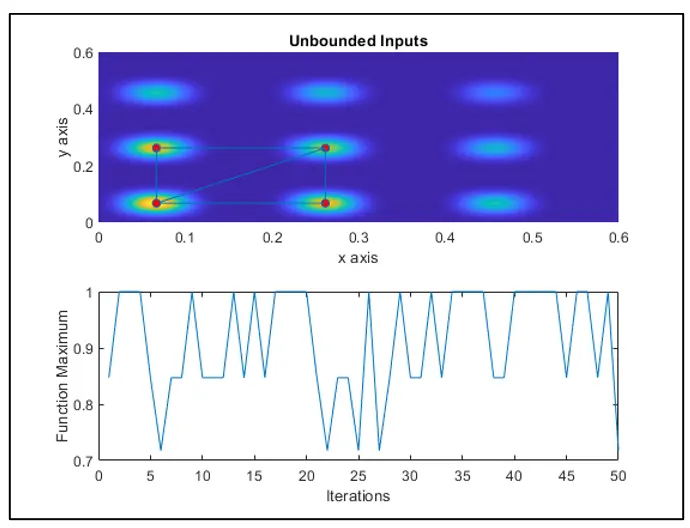
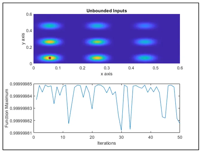
The three studies that were performed using the MATLAB code for the challenge purposes are attached in the following diagrams.

Study 1- Study the Genetic Algorithm for the random sampling

Study 2- Study the Genetic Algorithm with Upper and Lower Bound sampling

Study 3- Study the Genetic Algorithm with Upper and Lower Bound sampling and increase the population size

4 Conclusion:

In conclusion, the main aim of the week 4 challenge is to write a code in MATLAB to optimize the stalagmite function and find the global maxima of the function. In total, three studies were conducted to optimize or discover the value of the global maxima for the given stalagmite function. It was concluded that the study of the Genetic Algorithm with Upper and Lower Bound sampling with an increase in the population size was effectively able to calculate the global maxima for the given function.

References:

https://in.mathworks.com/help/gads/ga.html?searchHighlight=ga&s_tid=srchtitle_ga_1

https://in.mathworks.com/discovery/genetic-algorithm.html?s_tid=srchtitle_genetic%20algorithm_2

https://in.mathworks.com/help/gads/how-the-genetic-algorithm-works.html

5 Appendix:

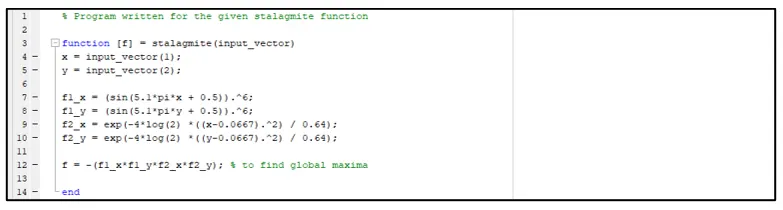
% Program written for the given stalagmite function

function [f] = stalagmite(input_vector)
x = input_vector(1);
y = input_vector(2);

f1_x = (sin(5.1*pi*x + 0.5)).^6;
f1_y = (sin(5.1*pi*y + 0.5)).^6;
f2_x = exp(-4*log(2) *((x-0.0667).^2) / 0.64);
f2_y = exp(-4*log(2) *((y-0.0667).^2) / 0.64);

f = -(f1_x*f1_y*f2_x*f2_y); % to find global maxima

end

clear all
close all 
clc

% Defining of Research Space
x = linspace(0,0.6,150);
y = linspace(0,0.6,150);

% Creating a 2Dimensional Mesh
[xx,yy] = meshgrid(x,y);
num_cases = 50;

% Evaluating the Stalagmite Function
for i = 1:length(xx)                      % starting of the loop
    for j = 1:length(yy)
        input_vector(1) = xx(i,j);
        input_vector(2) = yy(i,j);
        f(i,j)= stalagmite(input_vector);
    end
end                                       % ending of the loop



%************************************************************************


% Study 1 Statistical Behaviour for the random sampling

tic
for k = 1:num_cases
    [inputs, fval(k)] = ga(@stalagmite,2);
    xval(k)= inputs(1);
    yval(k)= inputs(2);
end

study1_time = toc    % calculating time to run first study

figure(1)
hold on 
grid on
surfc(xx,yy,-f)
shading interp
title('Stalagmite Plot')
xlabel('x axis')
ylabel('y axis')

figure(2)
subplot(2,1,1)
hold on
surfc(xx,yy,-f)
shading interp
plot3(xval,yval,-fval,'marker','o','markersize',5,'markerfacecolor','r')
title('Unbounded Inputs')
xlabel('x axis')
ylabel('y axis')
subplot(2,1,2)
plot(-fval)
xlabel('Iterations')
ylabel('Function Maximum')

%************************************************************************

% Study 2 Staistical Behaviour with increasing iteration of GA
tic
for l = 1:num_cases
    [inputs, fval(l)] = ga(@stalagmite,2,[],[],[],[],[0;0],[1;1]);
    xval(l)= inputs(1);
    yval(l)= inputs(2);
end

study2_time = toc               % calculating time to run second study

figure(3)
subplot(2,1,1)
hold on
surfc(xx,yy,-f)
shading interp
plot3(xval,yval,-fval,'marker','o','markersize',5,'markerfacecolor','r')
title('Unbounded Inputs')
xlabel('x axis')
ylabel('y axis')
subplot(2,1,2)
plot(-fval)
xlabel('Iterations')
ylabel('Function Maximum')

%************************************************************************

% Study 3 Staistical Behaviour with upper and lower bounds
options = optimoptions('ga');
options = optimoptions(options,'PopulationSize',300);

tic
for l = 1:num_cases
    [inputs, fval(l)] = ga(@stalagmite,2,[],[],[],[],[0;0],[1;1],[],[],options);
    xval(l)= inputs(1);
    yval(l)= inputs(2);
end

study3_time = toc               % calculating time to run third study

figure(4)
subplot(2,1,1)
hold on
surfc(xx,yy,-f)
shading interp
plot3(xval,yval,-fval,'marker','o','markersize',5,'markerfacecolor','r')
xlabel('x axis')
ylabel('y axis')
title('Unbounded Inputs')
subplot(2,1,2)
plot(-fval)
xlabel('Iterations')
ylabel('Function Maximum')

%************************************************************************