Week 4.1 - Genetic Algorithm

• Selection
• Crossover
• Mutation

Genetic algorithms simulate the process of natural selection which means those species who can adapt to changes in their environment are able to survive and reproduce and go to next generation. In simple words, they simulate “survival of the fittest” among individual of consecutive generation for solving a problem.

Advantages Of (GA) :

• A genetic algorithm is a local search technique used to find approximate solutions to Optimisation and search problems.
• It is an efficient, and effective techniques for both optimization and machine learning applications.
• It is widely-used today in business, scientific and engineering disciplines.

Syntax Of (GA) :

• x= ga(@func,nvars) - finds a local unconstrained minimum,x,to the objective function, fun. nvars is the dimension (number of design variables) of fun
• x= ga(@func,nvars,A,b,Aeq,beq,beq -finds a local minimum x to fun, subject to the linear equalities Aeq*x = beq and A*x<=b
• x= ga(@func,nvars,A,b,Aeq,beq,beq,lp,up)
• x= ga(@func,nvars,A,b,Aeq,beq,beq,lp,up,nonlcon,intcon,options)

A,b - Is A linear inequality constraints.

Aeq,beq - Is A equality constraints.

lb - Is A lower bound.

up - Is A upper bound.

nonlcon - Is A non-linear constraints.

intcon - Is A vector of the postive integers.

opction - Is A optmisation opction.

Stalagmite Function:

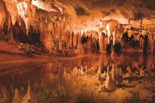
• A stalagmite is a type of rock formation that rises from the floor of a cave due to the accumulation of material deposited on the floor from ceiling drippings.
• Stalagmites are typically composed of calcium carbonate, but may consist of lava, mud, peat, pitch, sand, sinter, and ambera.
• A stalagmite function generally refers to the function with which we are generating values over a stalagmite kind of surface for finding out the local and global maxima and minima of that particular given function.

Here,

The equation of Stalagmite Function

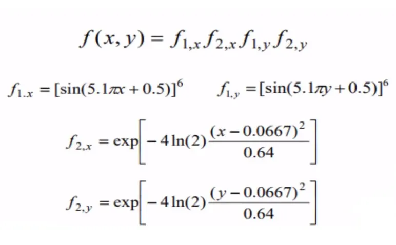
So ,I write the STALAGMITE FUNCTION.

FUNCTION PROGRAM:

function f = stalagmite_2(input_vector)

x = input_vector(1);
y = input_vector(2);

f1=(sin(5.1*pi*x+0.5))^6;
f2=(sin(5.1*pi*y+0.5))^6;
f3=exp((-4*log(2)*(x-0.0667)^2)/0.64);
f4=exp((-4*log(2)*(y-0.0667)^2)/0.64);

f = -(f1*f2*f3*f4);
end

Genetic Algorithm (GA) :

• Selection
• Crossover
• Mutation

Genetic algorithms simulate the process of natural selection which means those species who can adapt to changes in their environment are able to survive and reproduce and go to next generation. In simple words, they simulate “survival of the fittest” among individual of consecutive generation for solving a problem.

Syntax Of (GA) :

• x= ga(@func,nvars) - finds a local unconstrained minimum,x,to the objective function, fun. nvars is the dimension (number of design variables) of fun
• x= ga(@func,nvars,A,b,Aeq,beq,beq -finds a local minimum x to fun, subject to the linear equalities Aeq*x = beq and A*x<=b
• x= ga(@func,nvars,A,b,Aeq,beq,beq,lp,up)
• x= ga(@func,nvars,A,b,Aeq,beq,beq,lp,up,nonlcon,intcon,options)

The Genetic Process:

Genetic algorithms optimize by mimicking natural selection. GAs are different from artificial.neural networks in that the genetic process does not approximate a function, but is rather searching the solution space for an optimal solution. Just as nature doesn’t produce perfect organisms, GAs
have no guarantee to converge at the absolute maximum. In practice, however, GAs have been shown to work well for some applications.

MAIN PROGRAM :

close all
clear all
clc
num_cases=50;       % There is command on num of times (Ga) runs  

% Defining our search space
x = linspace(0,0.6,150);          % There is inputs of x axis
y = linspace(0,0.6,150);          % There is inputs of y axis

% Creating the 2Dimensional mesh
[xx yy]=meshgrid(x,y);            % There is a command of creating the 2d plot

% Evaluating the stalagmite function
for i=1:length(xx)
    for j=1:length(yy)
        input_vector(1)=xx(i,j);  
        input_vector(2)=yy(i,j);
        f(i,j)=stalagmite(input_vector);  % There is calling a stalagmite function
    end
end
surfc(x,y,f)       % There is a command on creating the 3d plot
xlabel('x axis')   % There is command on xlabel call axis
ylabel('y axis')   % There is command on xlabel call axis
shading interp     % There is a command on clear the shading on the plot

tic                % There is command on Start stopwatch timer

% Study 1 - unbounded condition.
% ga is in-built function.

for i=1:num_cases
   
[inputs,fopt(i)] = ga(@stalagmite,2);  % There command on (ga) find the local minimum  
xopt(i)=inputs(1);
yopt(i)=inputs(2);
end

study_time1=toc;   % There is command on end stopwatch timer

fopt=-fopt;
figure(1)
subplot(2,2,1)    % Subplot to help the plot specify value on plot
hold on           % There command on hold the previous plot
surfc(x,y,-f)
shading interp
plot3(xopt,yopt,fopt,'marker','o','MarkerSize',5,'MarkerFaceColor','r') % There is a command on how to expose plot on my inputs
title('un-bounded inputs')  % There is creating title on the plot
subplot(2,2,2)              % Subplot to help the plot specify value on plot
plot(fopt)
xlabel('itertions')         % There is a command on x axis call itertion
ylabel('function maxmum')   % There is a command on y axis call function maxmum


% Study 2 -Statistical behaviour with lower and upper bounds


tic

for i=1:num_cases
   
[inputs2,fopt2(i)] = ga(@stalagmite,2,[],[],[],[],[0,0],[1,1]);  % There is a command defines a set of lower and upper bounds on the design variable of (Ga)
xopt2(i)=inputs2(1);
yopt2(i)=inputs2(2);
end
study_time2=toc;

fopt2=-fopt2;
figure(2)
subplot(2,1,1)
hold on
surfc(x,y,-f)
shading interp
plot3(xopt2,yopt2,fopt2,'marker','o','MarkerSize',5,'MarkerFaceColor','r') % There is a command on how to expose plot on my inputs
title('unbound inputs')
subplot(2,1,2)
plot(fopt2)
xlabel('itertions')         % There is a command on x axis call itertion
ylabel('function maxmum')   % There is a command on y axis call function maxmum



% study 3 - Increasing GA Iterations
options=optimoptions('ga')
options=optimoptions(options,'PopulationSize',500);

tic
for i=1:num_cases
   
[inputs3,fopt3(i)] = ga(@stalagmite,2,[],[],[],[],[0,0],[0.6,0.6],[],[],options); % there is a command on
xopt3(i)=inputs3(1);
yopt3(i)=inputs3(2);

end

study_time3=toc;

fopt3=-fopt3;
figure(3)
subplot(2,1,1)
hold on
surfc(x,y,-f)
shading interp
plot3(xopt3,yopt3,fopt3,'marker','o','MarkerSize',5,'MarkerFaceColor','r')% There is a command on how to expose plot on my inputs
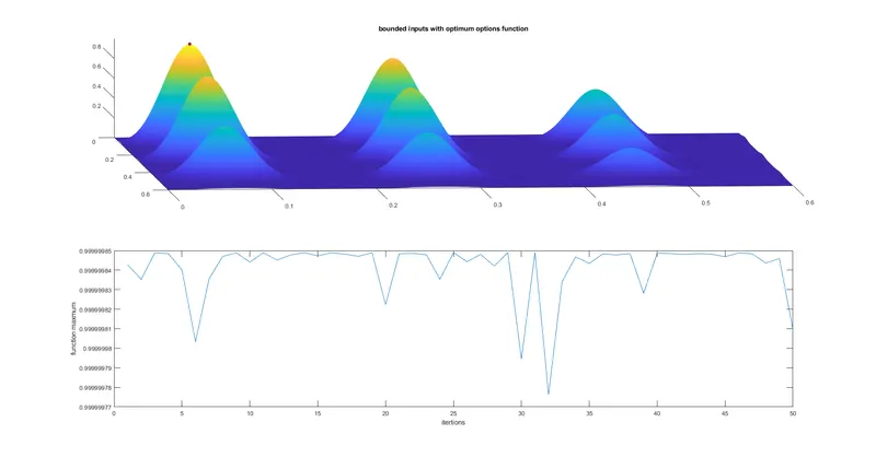
title('bounded inputs with optimum options function')
subplot(2,1,2)
plot(fopt3)
xlabel('itertions')        % There is a command on x axis call itertion
ylabel('function maxmum')  % There is a command on y axis call function maxmum

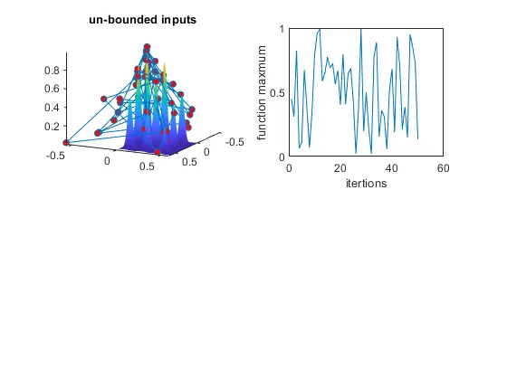
study_1

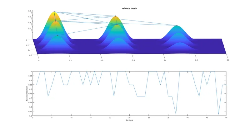
study_2

study_3

Reference:

https://www.mathworks.com/help/releases/R2022a/gads/ga.html#mw_9561d7b3-902b-481f-b95b-579424b64219

https://www.bing.com/ck/a?!&&p=6c47859b7669b6bed1d1b52e2889dcca96ed553cfa1282ce3568c3950df09892JmltdHM9MTY1MzgwNTc2NiZpZ3VpZD00NjVkMmExMC1iNWYzLTRjZDAtODUxMC02MjliYjVmMjU1ZmEmaW5zaWQ9NTAwMw&ptn=3&fclid=af9b0d13-df18-11ec-a101-fe291c992b1d&u=a1aHR0cHM6Ly93d3cubWF0aHdvcmtzLmNvbS9kaXNjb3ZlcnkvZ2VuZXRpYy1hbGdvcml0aG0uaHRtbA&ntb=1