Week 4.1 - Genetic Algorithm
AIM: - To writes a code in MATLAB to optimize the stalagmite function and to find the global maxima of the function and to explain the concept of genetic algorithm and its syntax in MATLAB.
GENETIC ALGORITHM: - Genetic algorithm is a search based optimization technique based on the principles of genetics and natural selection. It is frequently used to find optimal or near-optimal solutions. It is frequently used to solve optimization problems, in research, and in machine learning.
WORKING OF GENETIC ALGORITHM:-
The algorithm begins by creating a random initial population. The algorithm then creates a sequence of new populations. At each step, the algorithm uses the individuals in the current generation to create the next population.
Scores each member of the current population by computing its fitness value. These values are called the raw fitness scores. Scales the raw fitness scores to convert them into a more usable range of values. These scaled values are called expectation values.
Selects members, called parents, based on their expectation. Some of the individuals in the current population that have lower fitness are chosen as elite. These elite individuals are passed to the next population.
Produces children from the parents. Children are produced either by making random changes to a single parent—mutation—or by combining the vector entries of a pair of parents—crossover. Replaces the current population with the children to form the next generation.
Genetic Algorithm optimization starts with population initialization. Population is the number of sample data points taken to perform the genetic algorithm operation.
GA USED IN
Genetic Algorithms are used in optimization problems of various kinds, but they are frequently used in other application areas as well. The areas in which genetic algorithms are frequently used are listed below.
Optimization: - Genetic Algorithms are most commonly used in optimization problems wherein we have to maximize or minimize a given objective function value under a given set of constraints.
Economics: - GA are also used to characterize various economic models like the cobweb model, game theory equilibrium resolution, asset pricing, etc.
Neural Networks: - GA is also used to train neural networks, particularly recurrent neural networks.
Image Processing: - GA are used for various digital image processing(DIP) tasks as well like dense pixel matching.
SYNTAX AND EXPLANATION:-
- x = ga(fun,nvars) finds a local unconstrained minimum ,x, to the objective function fun. nvars is dimension (number of design variables) of fun.
- x = ga(fun,nvars,A,b) finds a local minimum x to fun, subject to the linear inequalities A*x≤ ga evaluates the matrix product A*x as if x is transposed(A*x’).
- x = ga(fun,nvars,A,b,Aeq,beq) finds a local minimum x to fun. Subject to the linear equalities Aeq*x = beq and A*x≤ (seta=[] and b=[] if no linear inequalities exist) ga evaluates the matrix product Aeq*x as if x is transposed(Aeq*x’).
- x = ga(fun,nvars,A,b,Aeq,beq,lb,ub) defines a set of lower and upper bounds on the design variables,x,so that a solution is found in the range lb≤x≤ub. (set Aeq = [] and beq = [] if no linear equalities exist.)
- x = ga(fun,nvars,A,b,Aeq,beq,lb,ub,noncom) subjects the minimization to the constraints define in nonlcon. The function nonlcon accepts x and returns vectors C and ceq, representing the nonlinear inequalities and equalities respectively. ga minimizes the fun nonlinear inequalities and equalities respectively. Ga minimizes the fun such that C(x)≤0 and Ceq(x) = 0. (Set lb = [] and ub = [] if no bounds exist.)
- x = ga(fun,nvars,A,b,Aeq,beq,lb,ub,nonlcon,options) minimizes with the default optimization parameters replaced by values in options.(Set nonlcon = [] if no nonlinear constraints exist.) Create options using optimoptions.
- x = ga(fun,nvars,A,b,Aeq,beq,lb,ub,nonlcon,lntcon) requires that the variables listed in lntCon take integer values.
- x = ga(problem) finds the minimum for problem, where problem is a structure.
- [x,fval] = ga(_ _) for any previous inputs arguments, also returns fval, the value of the fitness function at x.
- [x,fval,exitflag,output] = ga(_ _) also returns exitflag, an integer identifying the reason the algorithm terminated, and output, a structure that contains output from each generation and other information about the performance of the algorithm.
- [x,fval,exitflag,output,population,scores] = ga(_ _) also returns a matrix population, whose rows are the final population, and a vector scores, the scores of the final population.
PROGRAM DESCRIPTION:-
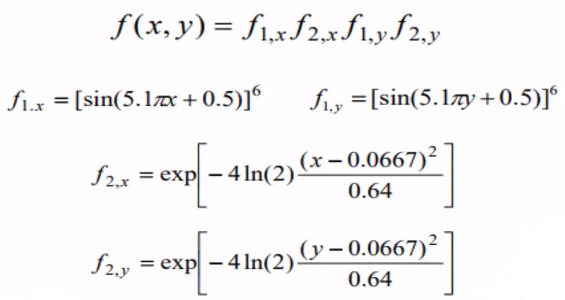
STALAGMITE FUNCTION: - Genetic algorithm is basically used to find Global minima value. Now our objective is to find the global maxima so we are going to add the negative sign in the stalagmite function and also in the surf command in the main program and this will be plotted in the positive quadrant of the graph. So we can find the global maxima value.
MATLAB CODE:-
clear all
close all
clc

%Defining our search space
x = linspace(0,0.6,150);
y = linspace(0,0.6,150);

num_cases = 50;
f1 = get_stalagmite(x,y);
F = -f1;

figure(1)
surfc(x,y,F)
xlabel('x value');
ylabel('y value');
shading interp

%Study 1 : Statistical behaviour
tic
for i = 1:num_cases
    [inputs, fopt(i)] = ga(@stalagmite,2);
    xopt(i) = inputs(1);
    yopt(i) = inputs(2);
end

study1_time = toc;
fopt = -fopt;

figure(2)

subplot(2,1,1)
hold on
surfc(x,y,F)
shading interp
plot3(xopt,yopt,fopt,'marker','o','markersize',5,'markerfacecolor','r')
title('unbounded inputs')
subplot(2,1,2)
plot(fopt)
xlabel('Iterations');
ylabel('Function maximum');

tic
%study_2 : Bounded inputs
tic
for i = 1:num_cases
    [inputs,fopt(i)] = ga(@stalagmite,2,[],[],[],[],[0;0],[0.5;0.5]);
    xopt(i) = inputs(1);
    yopt(i) = inputs(2);
end

study2_time = toc;
fopt = -fopt;
F = -f1;
figure(3)
subplot(2,1,1)
hold on
surfc(x,y,F)
shading interp
plot3(xopt,yopt,fopt,'marker','o','markersize',5,'markerfacecolor','r')
title('Bounded inputs')
subplot(2,1,2)
plot(fopt)
xlabel('Iterations');
ylabel('Function maximum');

%study 3 : Increased interations
options = optimoptions('ga');
options = optimoptions(options,'populationsize',170);

tic
for i = 1:num_cases
    [inputs, fopt(i)] = ga(@stalagmite,2,[],[],[],[],[0;0],[0.5;0.5],[],[],options);
    xopt(i) = inputs(1);
    yopt(i) = inputs(2);
end

study3_time = toc;
fopt = -fopt;
F = -f1;
figure(4)
subplot(2,1,1)
hold on
surfc(x,y,F)
shading interp
plot3(xopt,yopt,fopt,'marker','o','markersize',6,'markerfacecolor','r')
title('Increased Iterations')
subplot(2,1,2)
plot(fopt)
xlabel('Iterations');
ylabel('Function maximum');
STALAGMITE FUNCTION :-
function [f] = stalagmite(input_vector)

x = input_vector(1);
y = input_vector(2);

f1 = (sin(5.1*pi*x + 0.5)).^6;
f2 = exp(-4*log(2).*(((x -0.0667).^2)./0.64));
f3 = (sin(5.1*pi*y + 0.5)).^6;
f4 = exp(-4*log(2).*(((y -0.0667).^2)./0.64));

% negative sign is used to get the global maxima
f = -(f1.*f2.*f3.*f4);
end
GET_STALAGMITE FUNCTION:-
function [f1] = get_stalagmite(x,y)
[xx,yy] = meshgrid(x,y)

for i = 1:length(xx)
    for j = 1:length(yy)
        input(1) = xx(i,j);
        input(2) = yy(i,j);
        f1(i,j) = stalagmite(input);
    end
end
end
CODE PROCEDURE:-
Initially x and y range is given as 0 to 0.6 with range of 150 and num_cases is given as 60.
We will store the x,y value in a 2d array by using meshgrid function.
In the main program code x and y value is define by using the linspace command.
After that num_cases is fixed Num_cases =50, It is manialy used to check the consistency of the values we are getting in the plot.
After that first graph plot between the x,y and F. F is the function value.
Then I will be starting the first study. The Study behavior for the figure 2 with unbounded inputs includes calling our predefined function in a loop function and running it with our number of num_cases. The study time for plot is calculated and surface plot is employed here.
The study behavior for figure 3 with bounded inputs includes calling our predefined function as in study behaviour1. The only difference between 1 and 2 is, the plot 3 will have different syntax of ga such that it will define along with the range of inputs.
The study behavior for figure 4 with increase in options includes calling our predefined function as in both studies. The difference among all the three studies are, in the third study we increase the size.
RESULTS :-
GRAPH 1:-
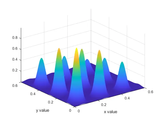
This graph is for the fitness function.
GRAPH2:-
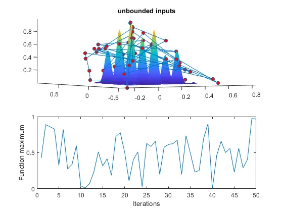
This is the graph is of study 1 Unbounded inputs.
GRAPH 3:-
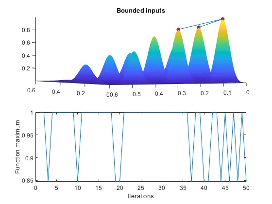
This is the graph of study 2 Bounded inputs.
GRAPH 4:-
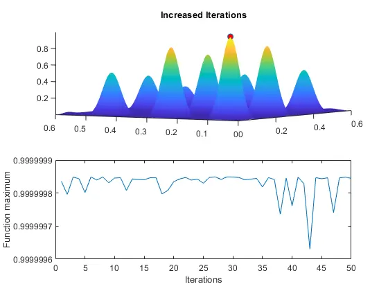
This is the graph of Study 3 increased Iteration.
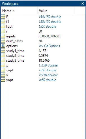
WORKSPACE WINDOW
CONCLUSION:-
Thus we have optimized stalagmite function and found the global maxima for the function.