Week 4.1 - Genetic Algorithm

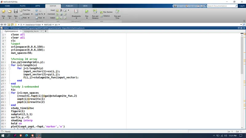
close all
clear all
clc
%input
x=linspace(0,0.6,150);
y=linspace(0,0.6,150);
num_spaces=50;

%forming 2d array
[xx,yy]=meshgrid(x,y);
for i=1:length(x)
for j=1:length(y)
input_vector(1)=xx(i,j);
input_vector(2)=yy(i,j);
f(i,j)=stalagmite_fun(input_vector);
end
end
%study 1-unbounded
tic
for i=1:num_spaces
[results,fopt(i)]=ga(@stalagmite_fun,2)
xopt(i)=results(1)
yopt(i)=results(2)
end
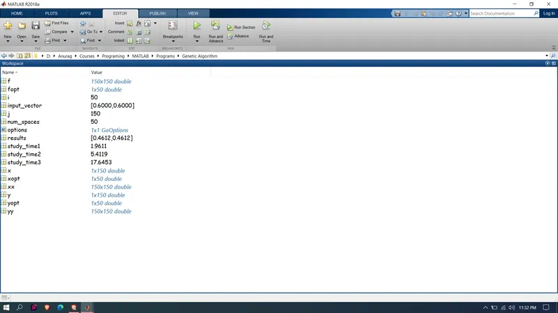
study_time1=toc
figure(1)
subplot(2,1,1)
surf(x,y,-f)
shading interp
hold on
plot3(xopt,yopt,-fopt,'marker','o')
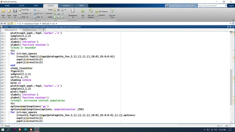
subplot(2,1,2)
plot(-fopt)
xlabel('iteration')
ylabel('function maximum')
%study 2- bounded
tic
for i=1:num_spaces
[results,fopt(i)]=ga(@stalagmite_fun,2,[],[],[],[],[0;0],[0.6;0.6])
xopt(i)=results(1)
yopt(i)=results(2)
end
study_time2=toc
figure(2)
subplot(2,1,1)
surf(x,y,-f)
shading interp
hold on
plot3(xopt,yopt,-fopt,'marker','o')
subplot(2,1,2)
plot(-fopt)
xlabel('iteration')
ylabel('function maximum')
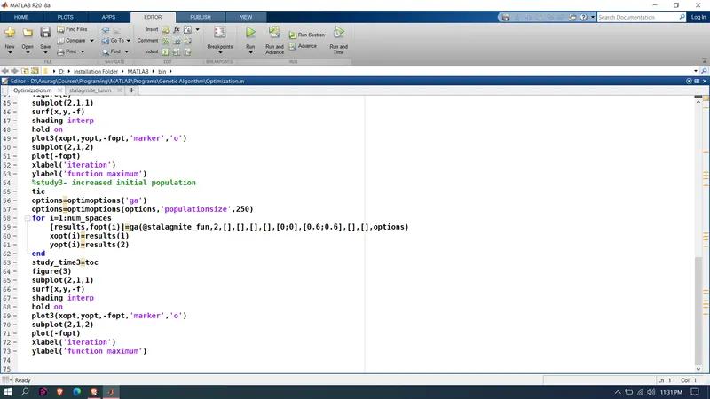
%study3- increased initial population
tic
options=optimoptions('ga')
options=optimoptions(options,'populationsize',250)
for i=1:num_spaces
[results,fopt(i)]=ga(@stalagmite_fun,2,[],[],[],[],[0;0],[0.6;0.6],[],[],options)
xopt(i)=results(1)
yopt(i)=results(2)
end
study_time3=toc
figure(3)
subplot(2,1,1)
surf(x,y,-f)
shading interp
hold on
plot3(xopt,yopt,-fopt,'marker','o')
subplot(2,1,2)
plot(-fopt)
xlabel('iteration')
ylabel('function maximum')

Explanation :-

First, we initialize the values of x and y taking 150 values between the interval 0 and 0.6

We consider no of iterations num_spaces=50.

Since we need to plot a 3D surface plot we take the 2d array of x and y using meshgrid command and store them in the input_vector array so that it can be used as an argument to call the function stalagmite

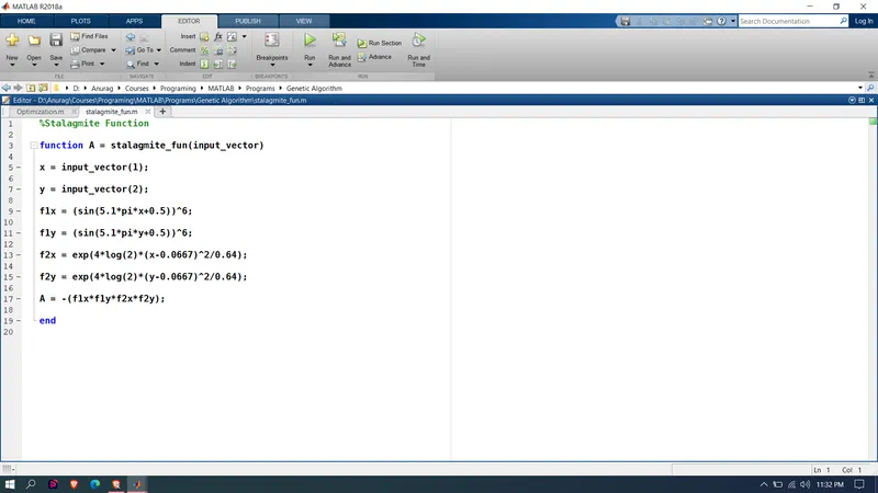
We create another function file for the stalagmite function. here we take the output as -f since ga only minimizes a given function.so if -f is considered it automatically gives us the maximas.

First study-

we take no of iterations = num_spaces and we use the genetic algorithm function to calculate the maxima of the function. we store the outputs into results that contain maxima and fopt which contain the value at which the maxima is obtained.

Here the ga is initiated with a random population.

We store the results into xopt, yopt. Now we need to plot the surface of x,y,-f to get the 3D plot.

We use the plot3 command to make a plot of xopt,yopt, and -fopt to plot the optimum maximas.

Also, plot the fopt function so that we can visualize the optimum values at each iteration.

To get the time taken to complete the cycle we used the tic toc commands to record the time.

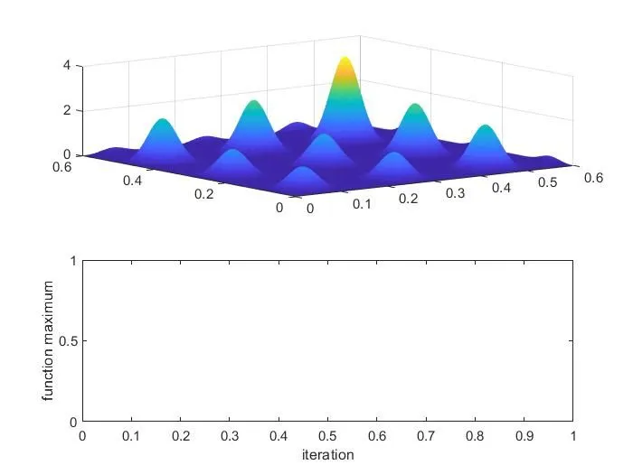
Here we can see the optimal values went outside the values of x and y resulting in falling away from the stalagmite surface.

So we failed to reach the global maxima in this case.

the study time = 2.4997s

Study having bounded values:-

Specify the lower and upper bounds of x and y in this case, the ga is initiated with a random population only.

store the results into xopt, yopt.now we need to plot the surface of x,y,-f to get the 3D plot.

We use the plot3 command to make a plot of xopt,yopt and -fopt to plot the optimum maximas.

Also, let us plot the fopt function so that we can visualize the optimum values at each iteration.

To get the time taken to complete the cycle we used the tic toc commands to record the time.

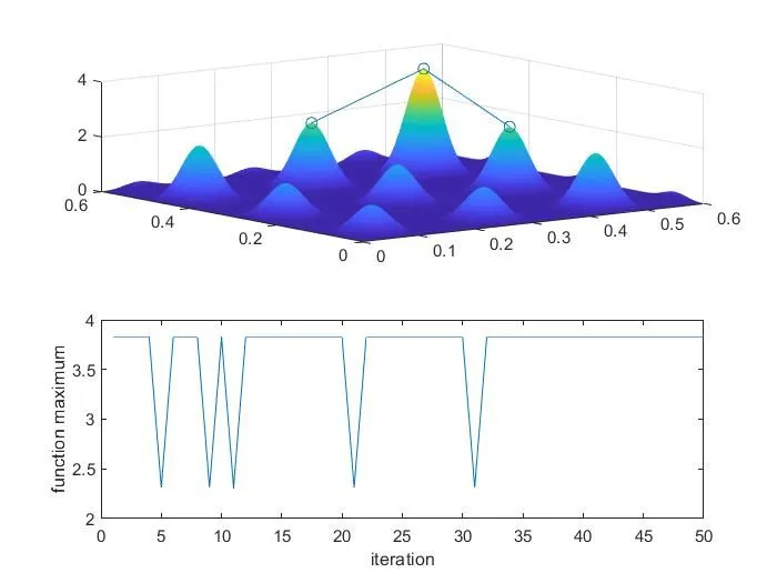
Though the optimum values are within the limits it could not give us the exact maxima values.

The study time = 3.3602s which is more than the above study.

A third study with initial population and bounded values-

Increase our initial population which is default as 50 to 250.

to set an initial population we need to use the command called optimum options and get our value of 'population size to 250.

now we store the results into xopt, yopt. Now we need to plot the surface of x,y,-f to get the 3D plot.

We use the plot3 command to make a plot of xopt,yopt and -fopt to plot the optimum maximas.

Also, let us plot the fopt function so that we can visualize the optimum values at each iteration.

To get the time taken to complete the cycle we used the tic toc commands to record the time.

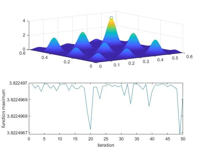
though the time of execution is more. In this case, we are successful to find out the correct maxima for the stalagmite function.

So by increasing the initial population size of the ga we can increase the accuracy of the algorithm.

The study time = 11.8696s which is more than the above two studies.

A Genetic Algorithm (GA) is a search-based optimization technique based on the principles of Genetics and Natural Selection. It is frequently used to find optimal or near-optimal solutions.

It is frequently used to solve optimization problems, in research, and in machine learning.

Genetic Algorithm optimization starts with population initialization,

The population is the number of sample data points taken to perform the genetic algorithm operation. These sample data points undergo the following three steps,

• Selection

In this step, the parents are selected from the sample data points, the main objective of the selection process is to select the highly fit individuals.

• Cross-Over

It is the process of taking two parents' solutions and producing the child from them.

• Mutation

The mutation is carried out to maintain the genetic diversity from one generation of a population of chromosomes to the next.

If a mutation is not performed, the chromosomes will become too similar to each other, convergence takes place soon and results in local minima.

Similar to the crossover, there are many ways to perform the mutation process.

• Fitness Function:

The fitness function takes the solution as input and produces the suitability of the solution as the output. This evaluates how close the solution is to the optimal solution of the desired problem.

Syntax for genetic algorithm-

we can give the inputs by any one of the following ways-

Description of input variables-

These are the various input syntaxes that can be given-