Project 2 - Rankine cycle Simulator

Main Code:-

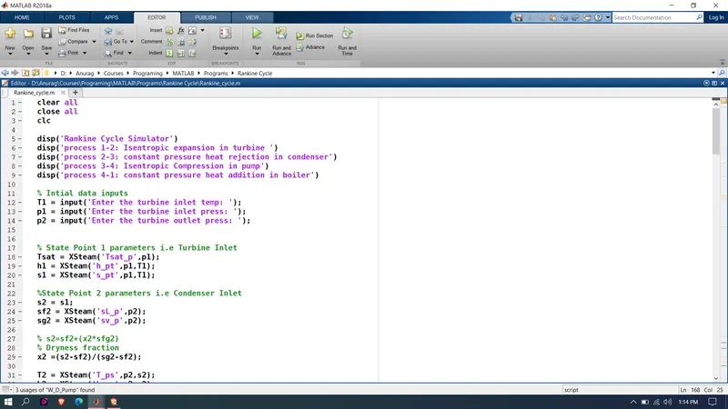
clear all
close all
clc

disp('Rankine Cycle Simulator')
disp('process 1-2: Isentropic expansion in turbine ')
disp('process 2-3: constant pressure heat rejection in condenser')
disp('process 3-4: Isentropic Compression in pump')
disp('process 4-1: constant pressure heat addition in boiler')

% Intial data inputs
T1 = input('Enter the turbine inlet temp: ');
p1 = input('Enter the turbine inlet press: ');
p2 = input('Enter the turbine outlet press: ');

% State Point 1 parameters i.e Turbine Inlet
Tsat = XSteam('Tsat_p',p1);
h1 = XSteam('h_pt',p1,T1);
s1 = XSteam('s_pt',p1,T1);

%State Point 2 parameters i.e Condenser Inlet
s2 = s1;
sf2 = XSteam('sL_p',p2);
sg2 = XSteam('sv_p',p2);

% s2=sf2+(x2*sfg2)
% Dryness fraction
x2 =(s2-sf2)/(sg2-sf2);

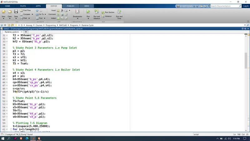
T2 = XSteam('T_ps',p2,s2);
h2 = XSteam('h_px',p2,x2);
hf2 = XSteam('hL_p',p2);

% State Point 3 Parameters i.e Pump Inlet
p3 = p2;
T3 = T2;
s3 = sf2;
h3 = hf2;
T5 = Tsat;

% State Point 4 Parameters i.e Boiler Inlet
s4 = s3;
p4 = p1;
h4=XSteam('h_ps',p4,s4);
cp=XSteam('cp_ps',p4,s4);
cv=XSteam('cv_ps',p4,s4);
c=cp/cv;
T4=T3*((p4/p3)^(c-1)/c)

% State Point 5,6 Parameters
T5=Tsat;
h5=XSteam('hL_p',p1);
s5=XSteam('sL_p',p1);
T6=T1;
h6=XSteam('hV_p',p1);
s6=XSteam('sV_p',p1);

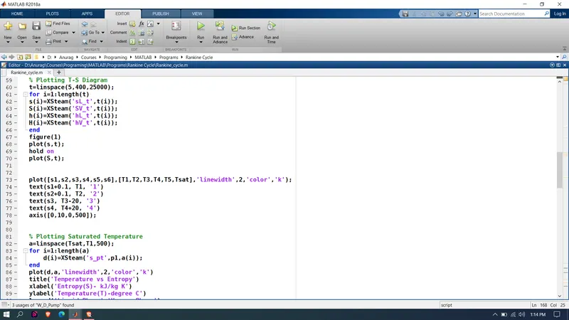
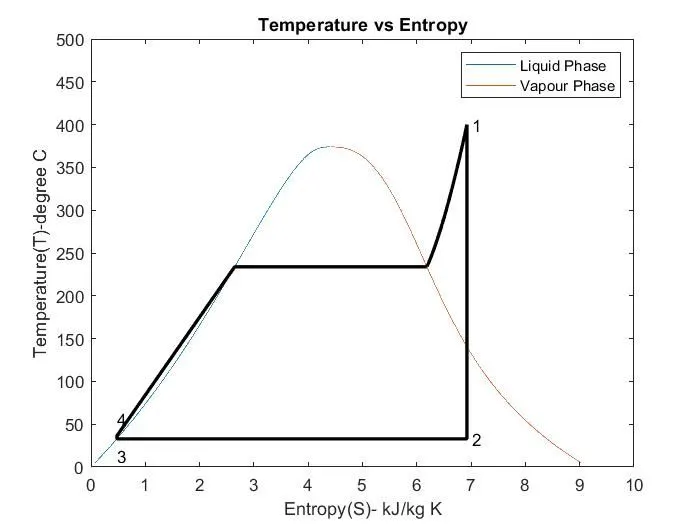
% Plotting T-S Diagram
t=linspace(5,400,25000);
for i=1:length(t)
s(i)=XSteam('sL_t',t(i));
S(i)=XSteam('SV_t',t(i));
h(i)=XSteam('hL_t',t(i));
H(i)=XSteam('hV_t',t(i));
end
figure(1)
plot(s,t);
hold on
plot(S,t);

plot([s1,s2,s3,s4,s5,s6],[T1,T2,T3,T4,T5,Tsat],'linewidth',2,'color','k');
text(s1+0.1, T1, '1')
text(s2+0.1, T2, '2')
text(s3, T3-20, '3')
text(s4, T4+20, '4')
axis([0,10,0,500]);

% Plotting Saturated Temperature
a=linspace(Tsat,T1,500);
for i=1:length(a)
d(i)=XSteam('s_pt',p1,a(i));
end
plot(d,a,'linewidth',2,'color','k')
title('Temperature vs Entropy')
xlabel('Entropy(S)- kJ/kg K')
ylabel('Temperature(T)-degree C')
legend('Liquid Phase','Vapour Phase')

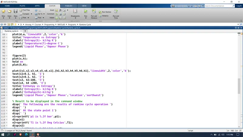
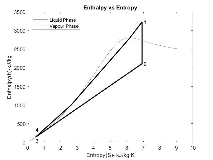
figure(2)
plot(s,h);
hold on
plot(S,H);

plot([s1,s2,s3,s4,s5,s6,s1],[h1,h2,h3,h4,h5,h6,h1],'linewidth',2,'color','k');
text(s1+0.1, h1, '1')
text(s2+0.1, h2, '2')
text(s3, h3-100, '3')
text(s4, h4 +200, '4')
title('Enthalpy vs Entropy')
xlabel('Entropy(S)- kJ/kg K')
ylabel('Enthalpy(h)-kJ/kg')
legend('Liquid Phase','Vapour Phase','location','northwest')

% Result to be displayed in the command window
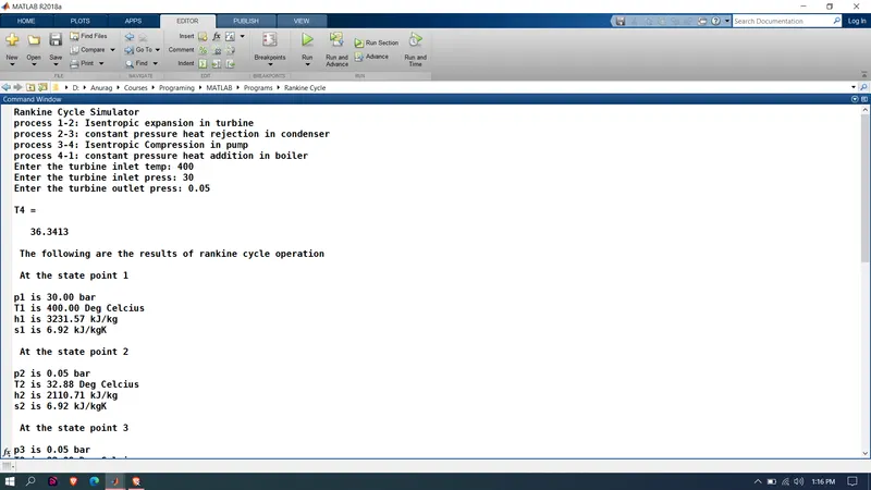
disp(' The following are the results of rankine cycle operation ')
disp(' ')
disp(' At the state point 1')
disp(' ')
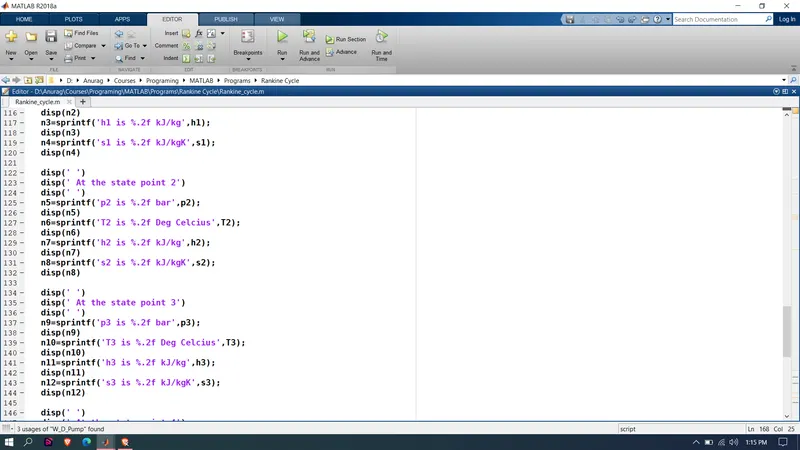
n1=sprintf('p1 is %.2f bar',p1);
disp(n1)
n2=sprintf('T1 is %.2f Deg Celcius',T1);
disp(n2)
n3=sprintf('h1 is %.2f kJ/kg',h1);
disp(n3)
n4=sprintf('s1 is %.2f kJ/kgK',s1);
disp(n4)

disp(' ')
disp(' At the state point 2')
disp(' ')
n5=sprintf('p2 is %.2f bar',p2);
disp(n5)
n6=sprintf('T2 is %.2f Deg Celcius',T2);
disp(n6)
n7=sprintf('h2 is %.2f kJ/kg',h2);
disp(n7)
n8=sprintf('s2 is %.2f kJ/kgK',s2);
disp(n8)

disp(' ')
disp(' At the state point 3')
disp(' ')
n9=sprintf('p3 is %.2f bar',p3);
disp(n9)
n10=sprintf('T3 is %.2f Deg Celcius',T3);
disp(n10)
n11=sprintf('h3 is %.2f kJ/kg',h3);
disp(n11)
n12=sprintf('s3 is %.2f kJ/kgK',s3);
disp(n12)

disp(' ')
disp(' At the state point 4')
disp(' ')
n13=sprintf('p4 is %.2f bar',p4);
disp(n13)
n14=sprintf('T4 is %.2f Deg Celcius',T4);
disp(n14)
n15=sprintf('h4 is %.2f kJ/kg',h4);
disp(n15)
n16=sprintf('s4 is %.2f kJ/kgK',s4);
disp(n16)

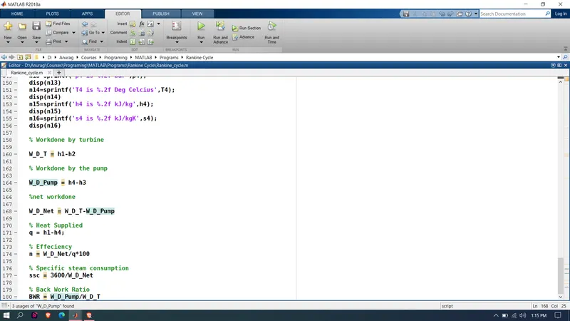
% Workdone by turbine

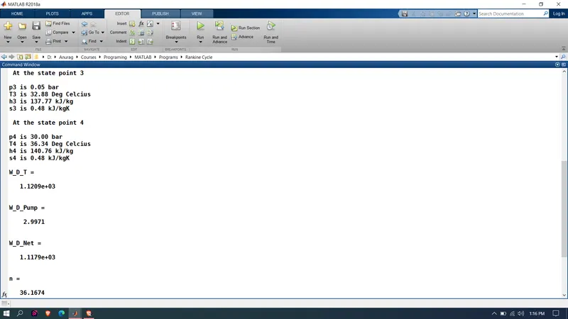
W_D_T = h1-h2

% Workdone by the pump

W_D_Pump = h4-h3

%net workdone

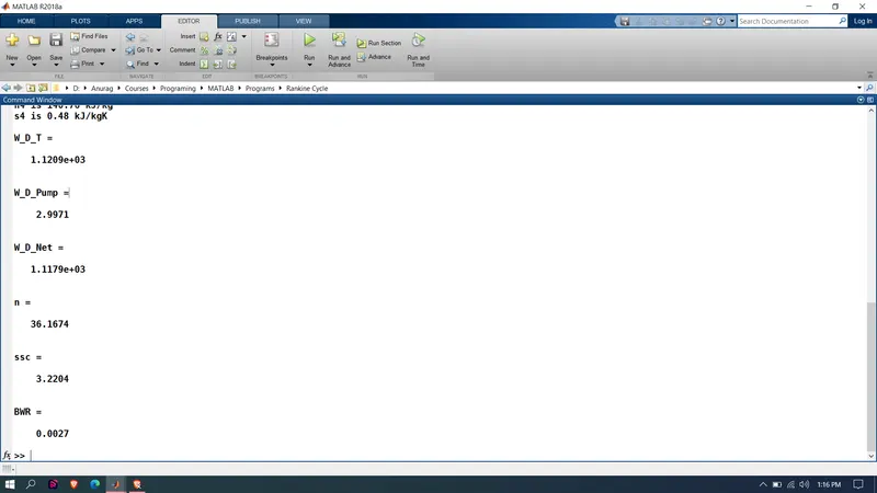
W_D_Net = W_D_T-W_D_Pump

% Heat Supplied
q = h1-h4;

% Effeciency
n = W_D_Net/q*100

% Specific steam consumption
ssc = 3600/W_D_Net

% Back Work Ratio
BWR = W_D_Pump/W_D_T

Step wise Explanation:-

Initially, we use the display command to display name of the program, and all the processes in the Rankine cycle each on a new line.

Then using the input command we take T1,p1,p2 as input from the user. Using this input and the XSteam file we find values of Tsat,h1 and s1. ie Turbine Inlet parameters.

Using p2 and XSteam file we find values of sf2 and sg2.

Using all values we calculate till now we find dryness fraction.

The with help of XSteam file we plot T2,h2, and hf2.

Then we define parameters for Pump Inlet

For values of Boiler Inlet (he, cp, cv) we again use XSteam.

Then calculate c and T4.

Using XSteam again we find values of state points 5 and 6.

Then using arrays and for loop, we plot T-S and saturated temperature plot.

The using disp command we display the results in the command window.

Now finally with all the values, we calculate the work done by Turbine as well as the pump and the net-work done. Along with Heat supplied, Efficiency, and Specific steam consumption, the Back work ratio.

Research done:-

Matlab documentation for syntax of some command. No research needed on the Rankine cycle as familiar with the concept of being a Mechanical Engineering Graduate.