Week 4.1 - Genetic Algorithm

What is GA?

Genetic Algorithm is an advanced process of optimization based on the Theory of Evolution & Survival of the Fittest by Charles Darwin, which is inspired by natural phenomenon such as selection, cross-over and mutation.

In GA,

• An initial population is subjected to recombinations such as selection, mutation and cross-overs.
• This gives rise to a new generation of children, which are again subjected to the above recombinations.
• The process continues till the same set of resuts repeats over and over which is known as the best result.

GA is highly randomiszed but performs better than local searches since they take into account past records.

Advantages of GA-

• Does not require derivative knowledge as it may not be available during optimization process.
• It is metahueristic, thus more effective and faster than traditional methods.
• Useful in searching vast population sizes.

Disadvantages of GA-

• It is not applicable to all problems, some functions fail when put through GA.
• Inputs need to be meticulous as false data may not give optimal solution.

We Aim to use GA to calculate the Global Maxima of the given Stalagmite Function.

• the Stalagmite Equation is defined as a function and the overall equation is multiplied by -1 as we require the Global Maxima (GA optimizes to give out Global Minima).
• In the main function-
  • c and y inputs are defined by 'linspace' command.
  • they are then converted into an array [xx yy] to plot the 3-dimensional surface plot
  • this array is put through the GA solver and the stalgmite function is called.
  • the total number of times GA runs is defined by num_cases and with the help of for loop all iterations are run and stored in an array.
  • the total study time is calculated using 'tic' and 'toc' commands.
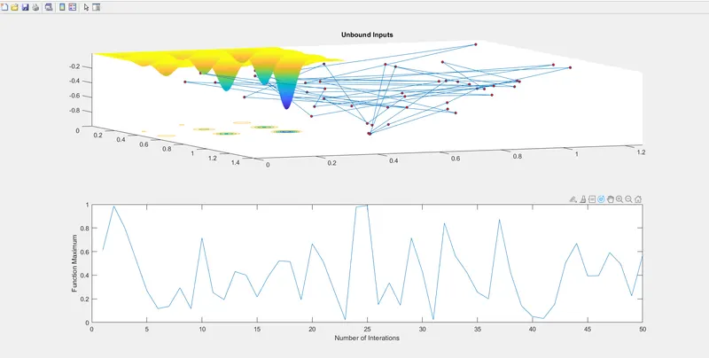
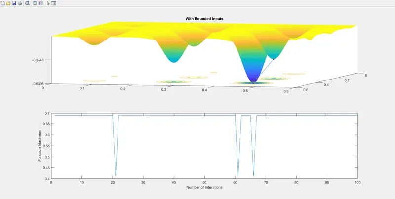
  • the results are plotted using 'surfc' and 'plot'.
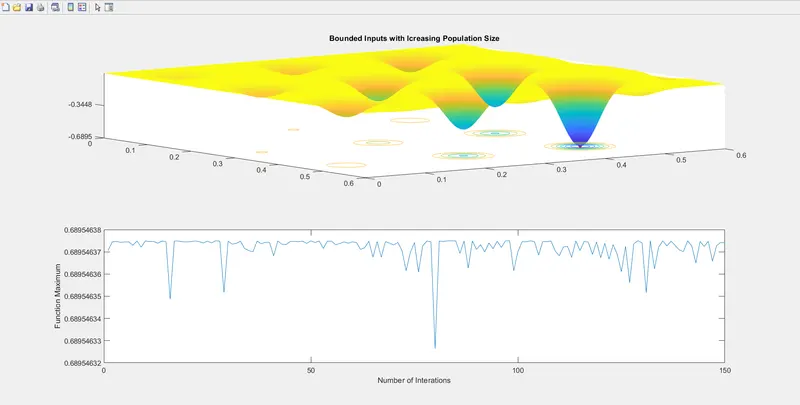
• GA is run 3 times with unbounded inputs, bounded inputs and bounded inputs with increasing population size.

GA Syntax-

The GA syntax is as follows-

• x = ga(fun,nvars,A,b,Aeq,beq,lb,ub,nonlcon,options)
• x is the local minima point for the given equation.
• fun is the function to be called.
• nvars is number of variables.
• A and b are any inequalities that exist in the function.
• Aeq and beq are also inequalitite.
• lb is lower bound.
• ub is upper bound.
• nonlcon gives 2 vectors representing inequalities and equalities.
• options is used to perform additional operations such as increasing population size which is done by 'optimoptions' (built in).

No major errors were encountered during the running of the function, only typing errors.

Stalagmite Function

function [f] = stalagmite_func(input_vector)

x = input_vector(1);
y = input_vector(2);
f1 = (sin(5.1*pi*x+0.5))^6;
f2 = (sin(5.1*pi*y+0.5))^6;
f3 = exp(-4*log(2)*(x-0.6667)^2/0.64);
f4 = exp(-4*log(2)*(y-0.6667)^2/0.64);
f = -(f1*f2*f3*f4);
end

First Iteration - Unbounded Inputs

clear all
close all
clc

x = linspace(0,0.6,150);
y = linspace(0,0.6,150);
[xx,yy] = meshgrid(x,y);

for i = 1:length(xx);
    for j = 1:length(yy);
        input_vector(1) = xx(i,j);
        input_vector(2) = yy(i,j);
 f(i,j) = stalagmite_func(input_vector);
    end
end

num_cases = 50;
tic
for i = 1:num_cases
    [inputs,f_opt(i)] = ga(@stalagmite_func,2);
    x_opt(i) = inputs(1);
    y_opt(i) = inputs(2);
    opt_f(i) = -f_opt(i);
end
study1_time = toc

subplot(2,1,1)
hold on
surfc(xx,yy,f)
shading interp 
plot3(x_opt,y_opt,-opt_f,'marker','o','markersize',4,'markerfacecolor','r')
title('Unbound Inputs')
subplot(2,1,2)
plot(opt_f)
xlabel('Number of Interations')
ylabel('Function Maximum')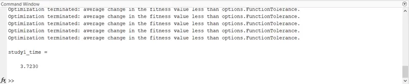

Seond Iteration - Bounded Inputs

clear all
close all
clc

x = linspace(0,0.6,150);
y = linspace(0,0.6,150);
[xx,yy] = meshgrid(x,y);

for i = 1:length(xx);
    for j = 1:length(yy);
        input_vector(1) = xx(i,j);
        input_vector(2) = yy(i,j);
 f(i,j) = stalagmite_func(input_vector);
    end
end

num_cases = 100;
tic
for i = 1:num_cases
    [inputs,f_opt(i)] = ga(@stalagmite_func,2,[],[],[],[],[0,0],[0.6,0.6]);
    x_opt(i) = inputs(1);
    y_opt(i) = inputs(2);
    opt_f(i) = -f_opt(i);
end
study2_time = toc

subplot(2,1,1)
hold on
surfc(xx,yy,f)
shading interp 
plot3(x_opt,y_opt,-opt_f,'marker','o','markersize',4,'markerfacecolor','r')
title('With Bounded Inputs')
subplot(2,1,2)
plot(opt_f)
xlabel('Number of Interations')
ylabel('Function Maximum')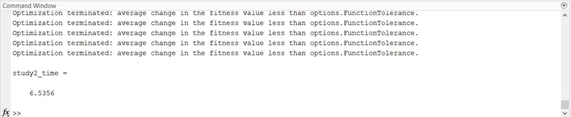

Third Iteration - Bounded Inputs with Increasing Population Size

clear all
close all
clc

x = linspace(0,0.6,150);
y = linspace(0,0.6,150);
[xx,yy] = meshgrid(x,y);

for i = 1:length(xx);
    for j = 1:length(yy);
        input_vector(1) = xx(i,j);
        input_vector(2) = yy(i,j);
 f(i,j) = stalagmite_func(input_vector);
    end
end

num_cases = 150;

options = optimoptions('ga');
options = optimoptions(options,'Populationsize',450);
tic
for i = 1:num_cases
    [inputs,f_opt(i)] = ga(@stalagmite_func,2,[],[],[],[],[0,0],[0.6,0.6],[],options);
    x_opt(i) = inputs(1);
    y_opt(i) = inputs(2);
    opt_f(i) = -f_opt(i);
end
study3_time = toc

subplot(2,1,1)
hold on
surfc(xx,yy,f)
shading interp 
plot3(x_opt,y_opt,-opt_f,'marker','o','markersize',4,'markerfacecolor','r')
title('Bounded Inputs with Icreasing Population Size')
subplot(2,1,2)
plot(opt_f)
xlabel('Number of Interations')
ylabel('Function Maximum')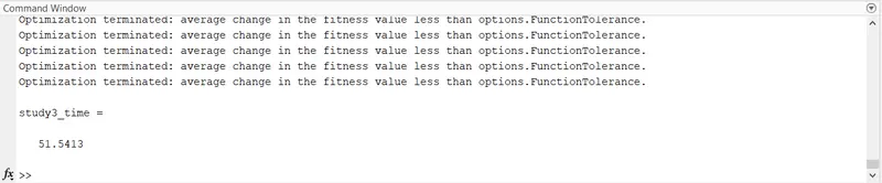

Result-

As we can see,

• during the first iteration, since there are no bounds the optimal points lie outside the function space.
• during the second iteration, as bounds are given the optimal points lie inside the finction space.
• and in the third iteration, the global maxima coverges on one single point.

So by limiting the search space and increasing the iterations(population) we can get the global maxima for the given Stalagmite Function.