Project 2 - Rankine cycle Simulator

clear all
close all 
clc

%display
disp('Rankine Cycle Simulator')
disp('1-2 isentropic expansion in turbine')
disp('2-3 constant pressure heat rejection by condenser')
disp('3-4 isentropic compression in the pump')
disp('4-1 constant pressure heat addition by the boiler')

%inputs
t_1 = input('enter the temp at turbine inlet (in °C):');
p_1 = input('enter the pressure at the turbine inlet (in bar):');
p_2 = input('enter the pressure at the turbine outlet (in bar):');

%turbine inlet temp = 400°C
%turbine inlet pressure = 30 bar
%turbine outlet pressure = 0.05 bar = condenser inlet pressure


%at state point 1
p1 = p_1;
t1 =  t_1;
s1 = XSteam('s_pT',p1,t1);
h1 = XSteam('h_pT',p1,t1);
ts1 = XSteam('Tsat_p',p1);
sf1 = XSteam('sL_p',p1);
sg1 = XSteam('sV_p',p1);
hf1 = XSteam('hL_p',p1);
hg1 = XSteam('hV_p',p1);

%at state point 2
s2 = s1;
p2 = p_2;
t2 = XSteam('Tsat_p',p2);
ts2 = XSteam('Tsat_p',p2);
sf2 = XSteam('sL_p',p2);
sg2 = XSteam('sV_p',p2);
hf2 = XSteam('hL_p',p2);
hg2 = XSteam('hV_p',p2);
x2 = ((s2-sf2)/(sg2-sf2));
h2 = hf2 +(x2*(hg2-hf2));

%at state point 3
p3 = p2;
t3 = t2;
s3 = XSteam('sL_p',p3);
v3 = XSteam('vL_p',p3);
hf3 = XSteam('hV_p',p3);
hg3 = XSteam('hL_p',p3);
sf3 = XSteam('sV_p',p3);
sg3 = XSteam('sL_p',p3);
x3 = ((s3-sf3)/(sg3-sf3));
h3 = hf3 +(x3*(hg3-hf3));

cp4 = XSteam('cpL_p',p3);
cv4 = XSteam('cvL_p',p3);
gamma = (cp4/cv4);
g = (gamma-1)/gamma;

%at state point 4
p4 = p1;
s4 = s3;
h4 = XSteam('h_ps',p4,s4);
t4 = t3*((p4/p3)^g);
wt = h1-h2;
wp = h4+h3;
wnet = wt-wp;
Qin = h1-h4;
Qout = h2-h3;
Ntherm = (wnet/Qin)*100;
s.s.c = 3600/wt;

temp  = linspace(1,400,500);
for i = 1:length(temp)
    a(i) = XSteam('hL_T',temp(i));
    b(i) = XSteam('hV_T',temp(i));
    c(i) = XSteam('sL_T',temp(i));
    d(i) = XSteam('sV_T',temp(i));
end

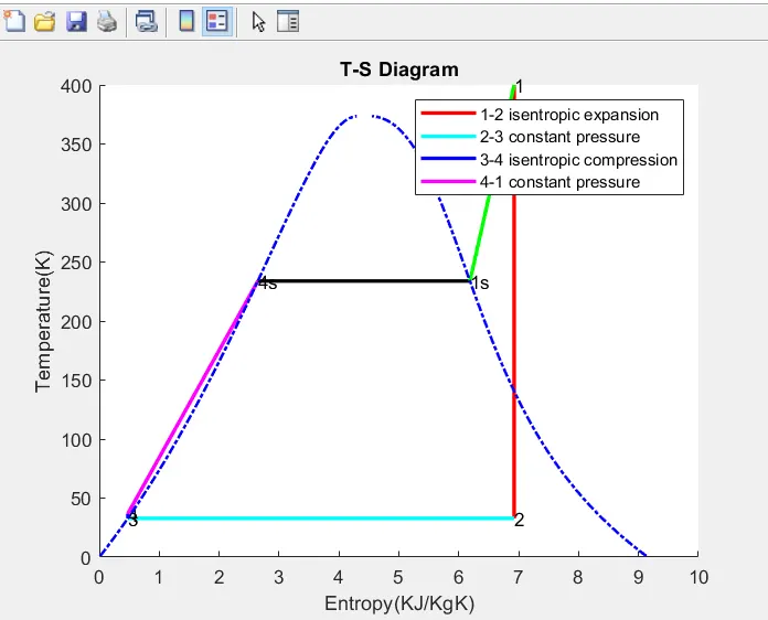
%plot 1
figure(1)
hold on
plot([s1 s2],[t1 t2],'color','r','linewidth',2)
text(s1,t1,'1')
text(s2,t2,'2')
plot([s2 s3],[t2 t3],'color','c','linewidth',2)
text(s3,t3,'3')
plot([s3 s4],[t3 t4],'color','b','linewidth',2)
text(s4,t4,'4')
plot([s4 sf1],[t4 ts1],'color','m','linewidth',2)
text(sf1,ts1,'4s')
plot([sf1 sg1],[ts1 ts1],'color','k','linewidth',2)
text(sg1,ts1,'1s')
plot([sg1 s1],[ts1 t1],'color','g','linewidth',2)
plot(c,temp,'color','b','linestyle','-.','linewidth',1.5)
plot(d,temp,'color','b','linestyle','-.','linewidth',1.5)
title('T-S Diagram')
xlabel('Entropy(KJ/KgK)')
ylabel('Temperature(K)')
legend('1-2 isentropic expansion','2-3 constant pressure','3-4 isentropic compression','4-1 constant pressure')

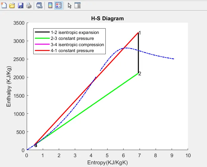
%plot 2
figure(2)
hold on
plot([s1 s2],[h1 h2],'color','k','linewidth',2)
text(s1,h1,'1')
plot([s2 s3],[h2 h3],'color','g','linewidth',2)
text(s2,h2,'2')
plot([s3 s4],[h3 h4],'color','m','linewidth',2)
text(s3,h3,'3')
plot([s4 s1],[h4 h1],'color','r','linewidth',2)
text(s4,h4,'4')
plot(c,a,'color','b','linestyle','-.','linewidth',1.5)
plot(d,b,'color','b','linestyle','-.','linewidth',1.5)
title('H-S Diagram')
xlabel('Entropy(KJ/KgK)')
ylabel('Enthalpy (KJ/Kg)')
legend('1-2 isentropic expansion','2-3 constant pressure','3-4 isentropic compression','4-1 constant pressure')

%display
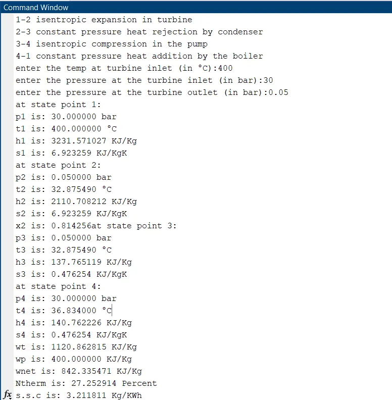
disp('at state point 1:')
fprintf('p1 is: %f bar\n',p1)
fprintf('t1 is: %f °C\n',t1)
fprintf('h1 is: %f KJ/Kg\n',h1)
fprintf('s1 is: %f KJ/KgK\n',s1)

disp('at state point 2:')
fprintf('p2 is: %f bar\n',p2)
fprintf('t2 is: %f °C\n',t2)
fprintf('h2 is: %f KJ/Kg\n',h2)
fprintf('s2 is: %f KJ/KgK\n',s2)
fprintf('x2 is: %f',x2)

disp('at state point 3:')
fprintf('p3 is: %f bar\n',p3)
fprintf('t3 is: %f °C\n',t3)
fprintf('h3 is: %f KJ/Kg\n',h3)
fprintf('s3 is: %f KJ/KgK\n',s3)

disp('at state point 4:')
fprintf('p4 is: %f bar\n',p4)
fprintf('t4 is: %f °C\n',t4)
fprintf('h4 is: %f KJ/Kg\n',h4)
fprintf('s4 is: %f KJ/KgK\n',s4)

fprintf('wt is: %f KJ/Kg\n',wt)
fprintf('wp is: %f KJ/Kg\n',t1)
fprintf('wnet is: %f KJ/Kg\n',wnet)
fprintf('Ntherm is: %f Percent\n',Ntherm)
fprintf('s.s.c is: %f Kg/KWh\n',s.s.c)

Steps-

• Start with 'clear all' 'close all' 'clc'.
• display the Rankine Cycle simulator and the steps involved in Rankine Cycle.
• input variables with 'input' command.
• now state wise we either define or derive the values required from the XSteam file.
• repeat for all states.
• calculate for gamma, work, thermal efficiency and SSC.
• for the saturation curve temp range is defined using 'linspace' command.
• plotting for both T-S and H-S curves are done using 'plot' command.
• using 'fprintf' to print results in the command window.

H-S Diagram

T-S Diagram

Rankine Cycle

It is an idealized thermodynamic cycle of a heat engine that converts heat into mechanical work while undergoing a phase change. The friction losses are neglected of the 4 components. The heat is supplied externally in a closed loop and water is usually used as a working fluid.

Four Components of Rankine Cycle

1. Pump
2. Boiler
3. Turbine
4. Condenser

Processes of Rankine Cycle

1-2 Isentropic Expansion (in Turbine)

2-3 Constant Pressure Heat Rejection (By Condenser)

3-4 Isentropic Compression (By Pump)

Constant Pressure Heat Addition (In Boiler)